Wien2k Pseudopotential Testing
©️ Copyright 2025 @ Liu Theory Lab
Author:
林子越 (Ziyue Lin) 📨
Date:2025-11-28
Lisence:This document is licensed under Attribution-NonCommercial-ShareAlike 4.0 International (CC BY-NC-SA 4.0) license.
I. Structure Optimization
First, create a new folder in the current directory, for example named vasp. In this folder, first perform multi-pressure point optimization. (Multi-pressure point optimization steps can be found in the VASP documentation. This document uses the vasp software for geometry optimization as preprocessing example)
II. Preparing Files
Three scripts: 0-Rename.sh, 1-sub.pbs, 2-job.sh
(All input files are in Wien2k_INPUT.rar)
chmod +x 0-Rename.sh, 2-job.sh (Grant permissions)
III. Script Contents
0-Rename.sh (depends on phonopy)
1-sub.pbs
2-job.sh
IV. Submitting Scripts
./0-Rename.sh
qsub 1-sub.pbs
./2-job.sh
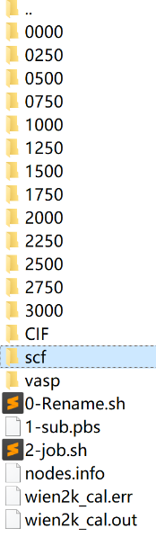
Output results are shown in the figure. After executing 0-Rename, a CIF folder is generated.
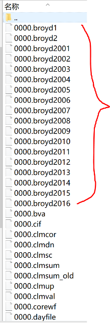
After submitting 1-sub.pbs, each pressure point will output a folder with many broyd files.
After executing 2-job.sh, an scf folder will be output containing the data needed for plotting.
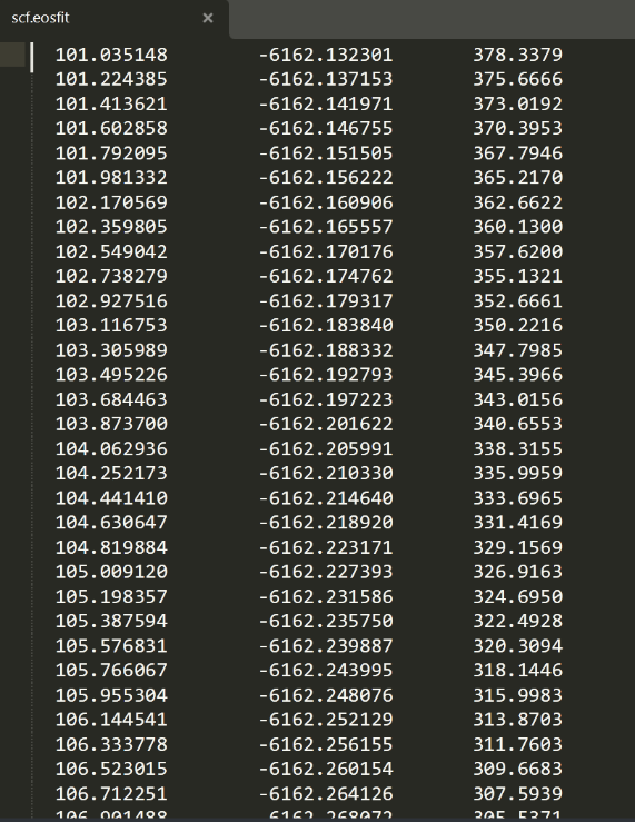
The file name for plotting is: scf.eosfit. As shown in the right figure, the first column is volume and the third column is pressure.
Pressure unit is GPa, volume conversion to cubic angstroms requires multiplying by 0.148187.
V. Linear Fitting
B-M equation of state E-V curve fitting tutorial:
http://blog.sciencenet.cn/blog-3388193-1152915.html
Click Tools - Fitting Function Generator
For fitting the P-V equation of state, the expression is:
x=(3/2)B0((V0/y)(7.0/y)-(V0/y)(5.0/3))(1+(3.0/4)(B1-4)*((V0/y)^(2.0/3)-1))
Where x is pressure, y is volume; parameters are B0, B1, V0.
Note: The above link's corresponding blog post is currently blocked and cannot access the specific content of the B-M equation of state E-V curve fitting tutorial. If you need to view related tutorials, it is recommended to contact the author or search for other resources.
The above link is invalid, see the tutorial below. Just look at the fitting section. In the AI era, using Python for fitting is recommended
Birch-Murnaghan Equation of State Fitting WIEN2k E-V Curve Tutorial
1. Introduction
In density functional theory (DFT) based first-principles calculations, by calculating the total energy (E) for a series of unit cell volumes (V), an energy-volume (E-V) curve can be obtained. The Birch-Murnaghan equation of state is a widely used empirical formula for fitting this E-V curve to extract material equilibrium physical properties at absolute zero, mainly including:
- Equilibrium volume \(V_0\)
- Equilibrium energy \(E_0\)
- Bulk modulus \(B_0\) (characterizes a material's ability to resist uniform compression)
- First-order pressure derivative of bulk modulus \(B_0'\)
This tutorial will guide you through the entire process from WIEN2k calculation to final fitting.
2. Basic Principle: Birch-Murnaghan Equation of State
The most commonly used form is the third-order Birch-Murnaghan equation of state, expressed as:
Where:
- \(E(V)\) is the total energy at volume \(V\).
- \(E_0\) is the ground state equilibrium energy (fitting parameter).
- \(V_0\) is the equilibrium volume (fitting parameter).
- \(B_0\) is the equilibrium bulk modulus (fitting parameter, unit usually GPa).
- \(B_0'\) is the first-order pressure derivative of \(B_0\) (fitting parameter, usually a dimensionless number between 3.5-5).
Simplified form (second-order): When \(B_0'\) is fixed at 4 (\(B_0''=0\)), the equation can be simplified to: $$ E(V) = E_0 + \frac{9V_0 B_0}{16} \left[\left(\frac{V_0}{V}\right)^{\frac{2}{3}} - 1\right]^2 \left{ 2 + \left[6 - 4\left(\frac{V_0}{V}\right)^{\frac{2}{3}}\right] \right} $$ The second-order form reduces one fitting parameter and is more stable when \(B_0'\) is close to 4 or when data points are few, but accuracy may be slightly lower. Generally, the third-order form is recommended.
3. WIEN2k Calculation Steps: Generating E-V Data Points
The core idea is: fix the unit cell shape and atomic positions, only uniformly scale the unit cell volume, perform self-consistent calculations at each volume, and extract total energy.
- Create initial structure: Use
structgenor import from crystal database to create an initial structure file (.struct) close to equilibrium. - Volume scaling:
- Determine a set of volume scaling factors (e.g., 0.94, 0.96, 0.98, 1.00, 1.02, 1.04, 1.06).
-
For each scaling factor \(c\), use the following command to scale lattice constants:
Note: For each different volume, you need to perform calculations in a separate directory to avoid file conflicts.
3. Execute calculations: - In the directory corresponding to each volume, execute standard WIEN2k self-consistent calculation loop:- Ensure each calculation reaches energy convergence (check the:ENEchange in the last line ofcase.scf). 4. Extract data: - After calculation completion, find the converged total energy (unit: Ry) from the last line ofcase.scffile in each directory. - Volume \(V\) can be calculated from lattice constants in.structfile (unit: \(a.u.^3\) or \(\AA^3\), ensure units are consistent). - Organize data into a two-column file (e.g.,eV_data.dat):
4. Fitting Methods
Method 1: Using Python (scipy.optimize.curve_fit)
This is a very flexible and powerful method.
Unit conversion note: The conversion factor 14710.5 in the above code applies when energy is in Ry and volume is in Bohr\(^3\) (a.u.\(^3\)). If your data units are different (such as eV and \(\AA^3\)), you need to use different conversion factors. This is one of the most error-prone areas in fitting.
Method 2: Using OriginLab or Gnuplot
These graphical software also support nonlinear fitting.
- Prepare data: Import
VandEtwo-column data into software. - Input equation: In nonlinear fitting tool, input third-order B-M equation formula.
-
Origin: Create a new function in Fitting Function Organizer, input a formula like the following (variable is x, parameters are E0, V0, B0, B0p):
- Gnuplot:3. Set initial parameters: Similar to Python code in Method 1, provide reasonable initial guess values (E0≈E_min,V0≈V@E_min,B0≈100-200,B0p≈4.0). 4. Execute fitting: Run iterative fitting, software will automatically find optimal parameters and their errors.
5. Results Analysis and Validation
- Graphical check: Always plot fitted curve and original data points! Ensure the curve passes through data points well, especially near the minimum (\(V_0\)).
- Parameter reasonableness:
$V_0$should be within your calculated volume range.$B_0$value should match known physical properties of the material you're studying (compare with literature). For example, ordinary metals typically have \(B_0\) between 50-200 GPa.$B_0'$is typically between 3.5 and 5.5.- Error assessment: Check standard errors of parameters given by fitting software. If a parameter's error is very large (e.g., error value comparable to parameter value itself), it indicates insufficient data to accurately determine that parameter, or initial guess value is too poor.
- Convergence: Ensure your WIEN2k calculations have sufficiently converged (
k-point grid,RKMAX,SCFiterations), otherwise data point noise will be large, affecting fitting accuracy.
6. Common Problems and Solutions
- Fitting doesn't converge or results are unreasonable:
- Problem: Initial guess values
(p0)are too far from true values. - Solution: Provide better initial values.
V0andE0can be estimated directly from data.B0can try a reasonable range (50, 100, 150...). B0error is very large:- Problem: Too few data points or volume range too narrow to constrain \(B_0\) (bulk modulus is second derivative of energy, requires high data precision).
- Solution: Add more volume points for calculation, especially near equilibrium volume \(V_0\).
- Unit errors:
- Problem:
B0fitting result value is 0.01 or millions, completely unreasonable. - Solution: Carefully check and unify all units (energy, volume), and perform correct unit conversion in equations. This is the most common problem!
By following these steps, you can reliably extract material equilibrium properties from WIEN2k calculation results.