Persistent Embryo Method and Landau-Ginzburg-Devonshire Model for Domain Nucleation¶

Author: Jiyuan Yang

In this tutorial I will show how to use revised Persistent Embryo Method (rPEM) to determine the critical nucleus during ferroelectric switching, and explain the Landau-Ginzburg-Devonshire (LGD) Model based on the results of molecular dynamics (MD) simulations.

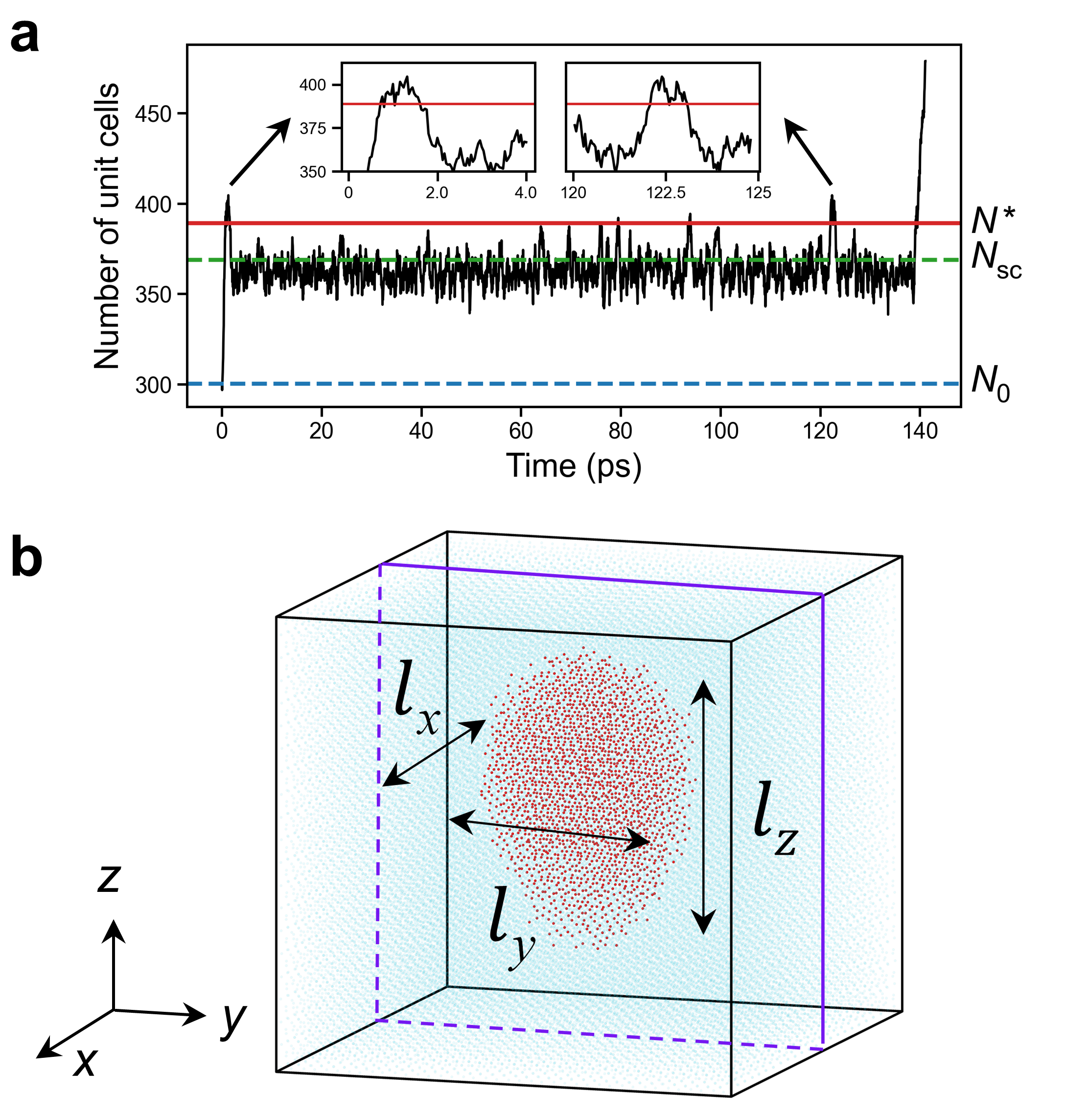
Traditional molecular dynamics simulations have limitations in capturing the nucleation of reversed domains under weak electric fields, as such events are extremely rare on accessible timescales. To address this issue, we employ PEM, originally developed for simulating three-dimensional (3D) crystal nucleation in liquids. Our improved version, termed the rPEM method, is specifically designed for simulating electric-field-driven nucleation in ferroelectrics. In the rPEM method, a 3D embryo consisting of $N_0$ reversed oxygen atoms (or unit cells) is first embedded within a single-domain structure.

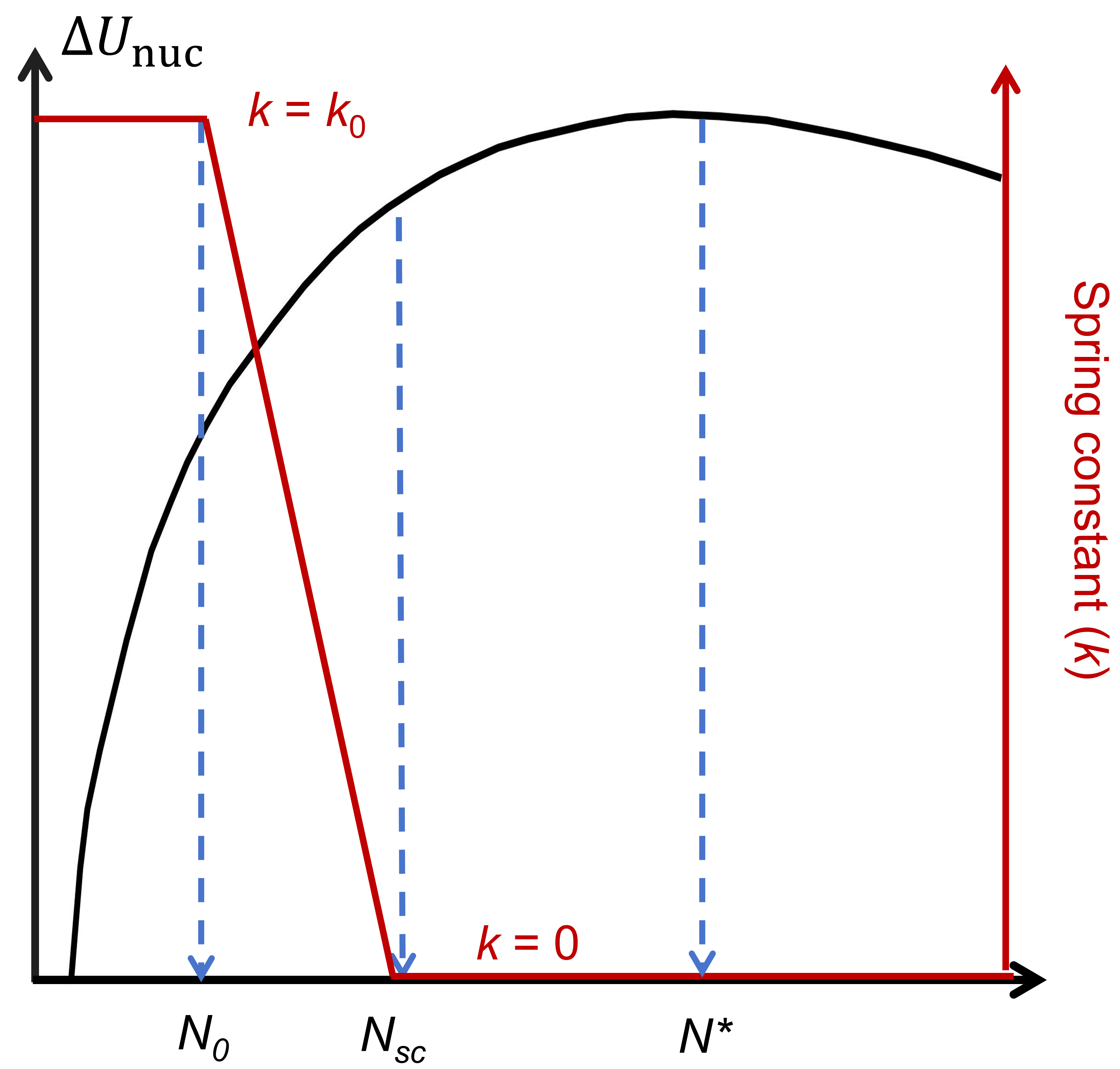
To prevent the system from reverting to its original state, an adjustable harmonic potential is applied to each oxygen atom in the embryo. This strategy effectively suppresses long-term nucleation fluctuations present in smaller nucleus. Once the nucleus size $N$ exceeds the subcritical threshold $N_{sc}$, the potential is gradually weakened and eventually removed. The elastic constant of the harmonic potential follows the formula $k(N) = k_0\left[(N_{\rm sc} - N)/N \right]$ (when $N < N_{\rm sc}$), otherwise $k(N) = 0$. By adaptively reducing the spring constant to zero before reaching the critical nucleus size, rPEM ensures that the system's dynamics at the critical point evolve naturally, i.e., without any bias. The observed plateau in the nucleus size evolution curve $N(t)$ indicates the period during which the nucleus size oscillates around $N^*$. These fluctuations allow us to determine the shape and size of the critical nucleus in an unbiased environment.

Take HfO$_2$ as an example, here I show the rPEM code for 3D nucleation.

# HfO2-efield

units           metal
boundary        p p p
atom_style      atomic

neighbor        2.0 bin
neigh_modify    every 10 delay 0 check no
# time unit ps
timestep     0.002

read_data   conf.lmp
#read_restart    E1.restart
#reset_timestep  0
mass            1 178.490000
mass            2 15.999400

#plugin load libdeepmd_lmp.so
#plugin load /path_to/dispplugin.so
plugin list

pair_style  deepmd  /path_to/ver5_compress.pb 
pair_coeff    * *

# set constant
# MD
variable        temp equal 300
variable        press equal 1.01325
variable        nloop equal 30000
# sprint constant k=kspr0*scaler, while scaler=(Nsc-Nsolid)/Nsc
variable        kspr0 equal 10.0
# *1ps, the time window to change the spring constant
variable        time_window equal 20 
variable        dump_window equal 20
variable        Nsc equal 1475
variable        Nbreak equal 5000
# cluster
variable        rcut equal 6.0
#seed region
variable       Xmin  equal  106.1208432556*15.0000000000/40.0
variable       Xmax  equal  106.1208432556*25.0000000000/40.0
variable       Ymin  equal  120.6758441164*19.0000000000/48.0
variable       Ymax  equal  120.6758441164*29.0000000000/48.0
variable       Zmin  equal  102.1310705291*10.0000000000/40.0
variable       Zmax  equal  102.1310705291*30.0000000000/40.0
#average displacement of layer24
variable      ave_disp_layer24   equal  1.0*0.54

variable HfID_h equal 38400
variable O1ID_h equal ${HfID_h}*2
variable O2ID_h equal ${HfID_h}*3

variable HfID_l equal 1
variable O1ID_l equal ${HfID_h}+1
variable O2ID_l equal ${O1ID_h}+1

group Hfall id ${HfID_l}:${HfID_h}
group O1all id ${O1ID_l}:${O1ID_h}
group O2all id ${O2ID_l}:${O2ID_h}

# group Hf delete 
# group O1 delete 
# group O2 delete 
# group fieldatoms delete

region field block INF INF INF INF INF INF 
group fieldatoms region  field

group Hf intersect Hfall fieldatoms
group O1 intersect O1all fieldatoms
group O2 intersect O2all fieldatoms
group O union O1 O2

# define seed group
region seedallR block ${Xmin} ${Xmax} ${Ymin} ${Ymax} ${Zmin} ${Zmax}
group seedall region seedallR
group seedO intersect seedall O
region Hfregion block INF INF ${Ymin} ${Ymax} INF INF 
group Hfregionatoms region Hfregion
group layer25 intersect Hfregionatoms O

# define initial position
compute displayer25 all customdisp   # calculting O displacement in the 4Hf cage
variable wx atom c_displayer25[1]
variable wy atom c_displayer25[2]
variable wz atom c_displayer25[3]

#move atoms in seed to make it is a real seed
displace_atoms seedO move 0.0 0.0 ${ave_disp_layer24}
write_data  initial+seed.data

# here updomain is the region which excludes seed
group updomain subtract all seedall
compute         scom seedall com
compute         scomHf    Hf  com

# update extended nuclear

variable   dnwz atom "v_wz >= 0.30"
group      dndomain dynamic all var dnwz every 1
compute        clustering dndomain cluster/atom ${rcut}
compute        cluster_index dndomain chunk/atom c_clustering
compute        cluster_size  dndomain property/chunk cluster_index count
variable        Ndndomain equal max(c_cluster_size)
#variable        Ndndomain equal count(dndomain)
thermo_style    custom step temp etotal pe ke press vol lx ly lz c_scom[1] c_scom[2] c_scom[3]  v_Ndndomain
run 0
print "ok"

# equilibrium updomain 
thermo      100

fix 1 updomain setforce NULL NULL NULL
fix 2 seedall setforce NULL NULL 0.0

min_style       cg
minimize            1.0e-10 1.0e-15 50000 100000

unfix 1
unfix 2

velocity all create ${temp} 23456789
fix equp updomain npt temp ${temp} ${temp} 1.0 z 1.0 1.0 5.0
fix    com_Hf   Hf   recenter INIT INIT INIT shift all
run 25000
unfix equp
unfix   com_Hf

write_data  Equ_updomain.data

# nucleation start
reset_timestep  0

# Apply field

variable VALUEX  equal 0
variable VALUEY  equal 0
variable VALUEZ  equal -0.025

variable Hffx equal 5.2*v_VALUEX
variable O1fx equal -2.6*v_VALUEX
variable O2fx equal -2.6*v_VALUEX

variable Hffy equal 5.2*v_VALUEY
variable O1fy equal -2.6*v_VALUEY
variable O2fy equal -2.6*v_VALUEY

variable Hffz equal 5.2*v_VALUEZ
variable O1fz equal -2.6*v_VALUEZ
variable O2fz equal -2.6*v_VALUEZ

fix             fHf  Hf addforce v_Hffx v_Hffy v_Hffz
fix             fO1  O1 addforce v_O1fx v_O1fy v_O1fz
fix             fO2  O2 addforce v_O2fx v_O2fy v_O2fz

# NPT
fix             ncl all npt temp ${temp} ${temp} 1.0 z 1.0 1.0 5.0
#fix             com_seed seedall recenter INIT INIT INIT shift all
#fix  rect  all  recenter  INIT  INIT  INIT
fix    com_Hf   Hf   recenter INIT INIT INIT shift all

# compute position
compute         uwpos all property/atom xu yu zu
#variable        px  atom c_uwpos[1]-c_scom[1]
#variable        py  atom c_uwpos[2]-c_scom[2]
#variable        pz  atom c_uwpos[3]-c_scom[3]
variable        px  atom c_uwpos[1]
variable        py  atom c_uwpos[2]
variable        pz  atom c_uwpos[3]
# store initial seeds' positions
fix             pseed0 seedall store/state 0 v_px v_py v_pz
variable        scaler equal 1.0

# loop starts
label           loop_mark
   variable        j loop ${nloop}
   variable        kspr equal ${kspr0}*${scaler}
   print           "LOOP= ${j} starts,  k= ${kspr}"
   variable        sprx atom 0
   variable        spry atom 0
   variable        sprz atom ${kspr}*(f_pseed0[3]-v_pz)

fix             spring seedall addforce v_sprx v_spry v_sprz  every 1
thermo_style    custom step temp etotal pe ke vol lx ly lz c_scom[1] c_scom[2] c_scom[3] v_Ndndomain v_kspr
run             ${time_window}

# update spring constant according to Ndndomain
variable        ss equal (${Nsc}-${Ndndomain})/${Nsc}
variable        scaler equal (${ss}>0)*${ss}
print           "LOOP= ${j} k= ${kspr} finished. Ndndomain= ${Ndndomain} Nsc= ${Nsc}"

# dump dndomain at the end of the loop 
#dump              trajdn dndomain custom  ${dump_window} ./traj/dn.*.atom id type x y z v_wx v_wy v_wz
#dump_modify       trajdn sort id
#dump              trajlayer25 layer25 custom  ${dump_window} ./traj/layer25.*.atom id type x y z v_wx v_wy v_wz
#dump_modify       trajlayer25 sort id
dump              trajall all custom  ${dump_window} ./traj/all.*.atom id type x y z v_wx v_wy v_wz
dump_modify       trajall sort id
run 0

if "${Ndndomain} > ${Nbreak}" then "jump  SELF break"
#undump     trajdn
#undump     trajlayer25
undump     trajall
unfix           spring
next            j
jump            SELF loop_mark

label           break

write_restart E2.restart

Then I will explain the key points in the code to make it easier to understand.

First you should install the plugin developed by Denan to enable displacement calculations in LAMMPS. The Github website for this plugin is: https://github.com/MoseyQAQ/liugroup-lammps-plugin.

Then use the following code to enable it in rPEM code:

1 2	`plugin load libdeepmd_lmp.so plugin load /path_to/dispplugin.so`

The required LAMMPS plugin for displacement calculations has been pre-installed on the GPU computing cluster maintained by Liu's research group (administered by Lintao). Users can directly access this implementation using the following code without additional installation steps.

1	`plugin list`

Then look at the MD settings: nloop determines when the rPEM algorithm terminates, kspr0 is the magnitude of the spring constant (driving force) that prevents back switching, time_window is the interval for adjusting kspr0. Nsc is the nucleus size when the driving force is canceled. Nbreak is the nucleus size used to determine complete reversal. The entire program stops when either Nbreak or nloop is reached. The rcut parameter determines the maximum interatomic distance for identifying atoms belonging to the same nucleus cluster. The initial reversed domain is defined within the spatial boundaries: X $\in$ (Xmin, Xmax), Y $\in$ (Ymin, Ymax), Z $\in$ (Zmin, Zmax). The ave_disp_layer24 parameter specifies the characteristic displacement distance for oxygen atoms during reversed domain construction.

To start, first construct a reversed nucleus:

1
2
3

#move atoms in seed to make it is a real seed
displace_atoms seedO move 0.0 0.0 ${ave_disp_layer24}
write_data  initial+seed.data

define the atoms not reversed:

1 2	`# here updomain is the region which excludes seed group updomain subtract all seedall`

Here we define the time-dependent size of nucleus on-the-fly, using the dynamic group:

# update extended nuclear

variable   dnwz atom "v_wz >= 0.30"
group      dndomain dynamic all var dnwz every 1
compute        clustering dndomain cluster/atom ${rcut}
compute        cluster_index dndomain chunk/atom c_clustering
compute        cluster_size  dndomain property/chunk cluster_index count
variable        Ndndomain equal max(c_cluster_size)

Then we perform a quick energy minimization step to optimize the atomic configuration containing the initial nucleus structure.

# equilibrium updomain 
thermo      100

fix 1 updomain setforce NULL NULL NULL
fix 2 seedall setforce NULL NULL 0.0

min_style       cg
minimize            1.0e-10 1.0e-15 50000 100000

unfix 1
unfix 2

velocity all create ${temp} 23456789
fix equp updomain npt temp ${temp} ${temp} 1.0 z 1.0 1.0 5.0
fix    com_Hf   Hf   recenter INIT INIT INIT shift all
run 25000
unfix equp
unfix   com_Hf

write_data  Equ_updomain.data

After routinely applying the electric field, we have completed all preparations to initiate the rPEM cycle. First, save the state of the initial seed.

# compute position
compute         uwpos all property/atom xu yu zu
#variable        px  atom c_uwpos[1]-c_scom[1]
#variable        py  atom c_uwpos[2]-c_scom[2]
#variable        pz  atom c_uwpos[3]-c_scom[3]
variable        px  atom c_uwpos[1]
variable        py  atom c_uwpos[2]
variable        pz  atom c_uwpos[3]
# store initial seeds' positions
fix             pseed0 seedall store/state 0 v_px v_py v_pz
variable        scaler equal 1.0

apply spring force:

1 2	`variable sprz atom ${kspr}*(f_pseed0[3]-v_pz) fix spring seedall addforce v_sprx v_spry v_sprz every 1`

update spring constant at every loop:

# update spring constant according to Ndndomain
variable        ss equal (${Nsc}-${Ndndomain})/${Nsc}
variable        scaler equal (${ss}>0)*${ss}
print           "LOOP= ${j} k= ${kspr} finished. Ndndomain= ${Ndndomain} Nsc= ${Nsc}"

Then we can dump the trajectory of nucleus evolution in every loop until the program terminates. These trajectories can be used to analyze the shape and boundary of the nucleus. Here is key information of the output of rPEM code:

1	`LOOP= 5 k= 1.76271186440678 finished. Ndndomain= 1227 Nsc= 1475`

use following code to extract it from lmp.log file then plot the data:

CURRENT=`pwd`
rm -rf results
mkdir results
grep -a LOOP lmp.log | grep Ndndomain | awk '{print $2, $4, $7}' > $CURRENT/results/tN_D1.dat

LGD 3D nucleation model¶

Based on the shape of nucleus from MD simulations, we can build a LGD model:

$\Delta U_{\rm nuc} = -\frac{\pi}{3}l_x^2l_z\eta P_s\mathcal{E}+\int_{0}^{2\pi}\mathrm{d}\varphi\int_{0}^{\pi}\sigma_x\sqrt{\sin^2\theta+\left(\frac{\sigma_z}{\sigma_x}\right)^2\cos^2\theta}~(l_\theta/2)^2\sin\theta\mathrm{d}\theta$

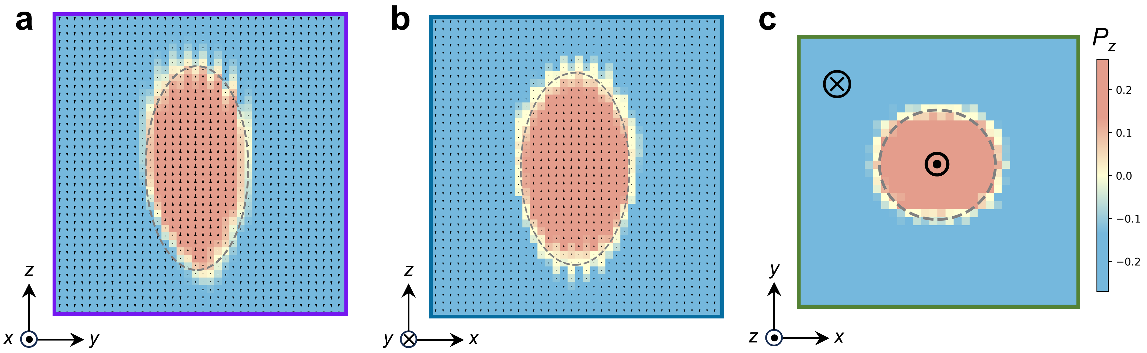
The details of this model can be found in PHYSICAL REVIEW X 15, 021042 (2025). Here I will use simple words to help readers understand the physical meaning of this model. Let us first look at the fully reversed (red) region. This region possesses the same energy as the initial blue region, meaning it incurs no additional energy penalty. Its sole effect is to reduce the total energy of the entire system by the following amount:

$\Delta U_{\mathrm{V}} = - \mathcal{E} \eta \iiint_V\mathrm{d}V \left (P_z^{\rm nuc}(x,y,z)-P_z^{\rm SD}(x,y,z) \right)$

Then look at the yellow region (the shell of nucleus). This region deviates from the system's energy optimum, thus incurring an energy penalty. The energy increase caused by the creation of these new surfaces can be expressed by the following equation:

$\Delta U_{\mathrm{I}} =\iint_{S}\sigma_\theta\mathrm{dS}$ where $\sigma_\theta$ is a spatial dependent surface energy along the shell.

So the energy of nucleus is the sum of these two energies:

$\Delta U_{\mathrm{nuc}}=\Delta U_{\mathrm{V}}+\Delta U_{\mathrm{I}}$

Note that this model is a zero-kelvin model, we need to extend it to finite temperature.

Use the method developed in Supplemental Material of PHYSICAL REVIEW X 15, 021042 (2025), we have:

$\sigma_\theta = \frac{8P_s}{3}\sqrt{g_{\theta}K_\mathrm{loc}}$

Therefore, the whole equation in fact is a function of $P_s$. Note that we have the temperature dependent polar mode from Landau phase transition theory:

$P_s(T)=\sqrt{\frac{T_c-T}{T_c}}P_s$

So the free energy is conveniently calculated using a temperature dependent polar mode.

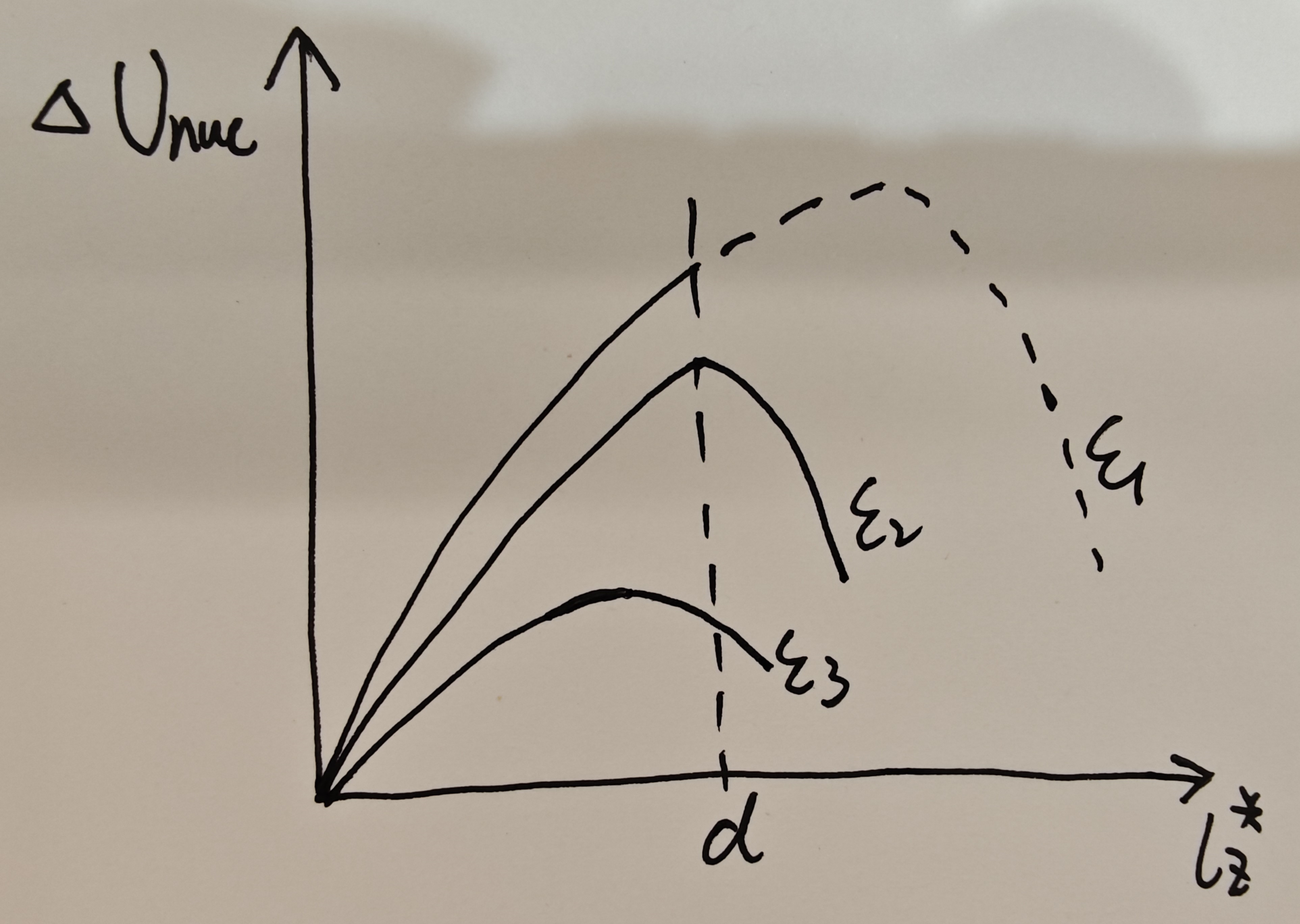
At a give electric field $\mathcal{E}$ , our LGD model fast predicts the critical size $𝑙_𝑧^∗(\mathcal{E})$ by calculating saddle point of $\Delta U_{\mathrm{nuc}}(T)$.

This physical quantity measures the ease of nucleation. Consider a film with a thickness of d. When a low electric field $\mathcal{E}_1$ is applied, the entire spatial extent of the film is insufficient to allow the system to reverse within the experimental timeframe. Only when the electric field is sufficiently large (e.g., $\mathcal{E}_3$) can nucleation and reversal occur within the thickness d. Thus, the coercive field is determined by the critical field when $𝑙_𝑧^∗(\mathcal{E}_c)≈𝑑$.