Structural optimization and band structure calculations using PWmat
©️ Copyright 2025 @ Liu Theory Lab
Author:
樊迪 (Di Fan) 📨
Date:2025-8-4
Lisence:This document is licensed under Attribution-NonCommercial-ShareAlike 4.0 International (CC BY-NC-SA 4.0) license.
1 Introduction
PWmat is a density functional theory (DFT) simulation software that runs on graphics processing units (GPUs) Item [1,2], which uses the plane wave pseudopotential method to support electronic structure, structural relaxation, ab initio molecular dynamics Multiple basic computational functions such as transition state search, real-time time-dependent density functional, and non adiabatic molecular dynamics. Simply put, there are three steps to using PWmat: 1. Prepare the input file; 2. Run PWmat; 3. Post processing and visualization.
Users need to prepare three types of input files: 1. Pseudo potential file: Only supports mode conservative pseudo potential and ultra soft pseudo potential. Users can download the pseudo potential package from the PWmat official website. If the structure to be calculated contains several elements, it is necessary to copy the pseudopotential files of these elements to the calculation directory; 2. Structure file: It must be in the format specified by PWmat, and users can use the structure conversion tool on the terminal Convert common crystal structure formats such as. cif and. xsf to PWmat format; 3. Parameter file: must be named etot.input, which specifies the names of the pseudopotential file and structure file, and Parameters such as truncation energy and k-point can be set.
2 Lattice optimization and atomic relaxation calculation
Different relaxation requirements are mainly achieved by modifying the parameters of atom.config and etot.input files. Example: * (Fixed) lattice optimization and atomic relaxation * (Partial) atomic relaxation * Optimization of electrified system
Step 1. Main input files:
atom.config:
Note: Two dimensional materials can be optimized by fixing the lattice, which can be set in atom.config
etot.input
Partial atomic relaxation:
atom.config:
RELAX_DETAIL=IMTH NSTEP FORCE_TOL ISTRESS TOL_STRESS 1. IMTH represents optimization methods
- IMTH=1(default),conjugated gradient;
- IMTH=2,BFGS method;
- IMTH=3,steepest decent;
- IMTH=4,preconditioned conjugate gradient;
- IMTH=5,Limited-memory BFGs method;
- IMTH=6,FIRE: Fast Inertial Relaxation Engine.
-
NSTEP represents the maximum number of relaxation steps
-
FORCE_TOL represents the convergence criterion for relaxation (eV/Å)
-
ISTRESS indicates whether lattice optimization is performed
-
TOL STRESS represents the standard for lattice optimization (eV/Natom)
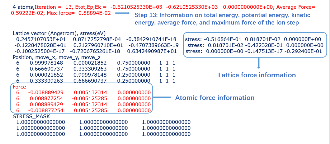
Step 2. Main output files:
- final.config: Relaxed structure
- RELAXSTEPS: RELAX per step
- MOVEMENT: Trajectory
final.config:
RELAXSTEPS:
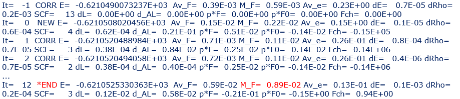
- It: The number of steps for ion optimization
- NEW: represents a change in the search direction of the step force; CORR: indicates that the search direction of the step force is consistent with the direction of the NEW step on it
- E: The total energy of the ion step system
- AV_F: The average force exerted on each atom in this step
- M_F: The maximum force exerted on all atoms in this step
- DE, dRho: The absolute value of the difference between the last step of the ion step that is self consistent and the previous step
- SCF: The number of autonomous steps included in the ion step
- dL: Step size of ion step movement
- p*F: Projection value of atomic force along the search direction
Note: If * END appears in the last step, it means that normal operation has ended
Extract column data from RELAXSSTEP and view the convergence information of the relaxation process (separated by spaces)
Method 1: Draw using the gnuplot command (enter gnuplot first to enter command-line mode)
Enter gnuplot to enter command-line mode
MOVEMENT:
You can convert MOVEMENT to an. xsf format file to view the relaxed trajectory animation Command line:
3 band structure calculations
- Perform self consistent computation first, followed by non autonomous computation (job=nonsref)
- When using HSE functional calculations, K-point parallel settings cannot be used
Step 1. Self consistent calculation (job=scf):
etot.input:
After the calculation is completed, keep OUT.FERMI and copy the potential file "OUT.VR" to "IN.VR“
Step 2. __ Prepare the high symmetry K-point file IN.KPT required for non autonomous computation__:
2.1 Generate k points based on the path of high symmetry points, create a gen.kpt file, write the coordinates of high symmetry points and the number of inserted points
gen.kpt:
2.2 Generate IN.KPT file after running the command, command line:
Prepare parameter files for non autonomous calculation:
etot.input:
Result post processing
Run plot band structure.x to generate bandstructure 1.txt
Command line:
plot band structure.x
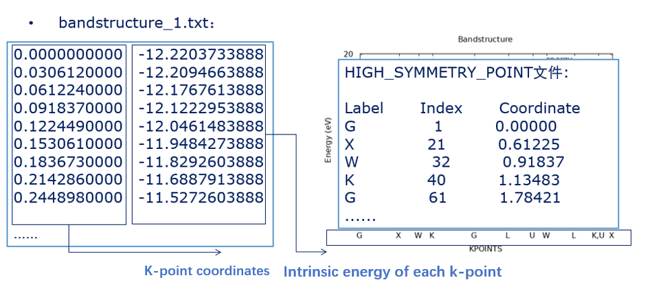
After pwmat completes the nonscf calculation, if there is an out.fermi file in the calculation directory, the txt and pictures obtained after running the script will reset the Fermi level to zero. In addition, if there is a report file, you can also use the gap read script to quickly calculate the band gap If there is further need, you can visit https://www.pwmat.com/pwmat-resource/Manual.pdf and https://www.pwmat.com/Tutorials to obtain the pwmat manual and tutorials.