Simulation of frequency-dependent dielectric spectra

©️ Copyright 2025 @ Yao Wu
Author： Yao Wu 📨
Date：2025-10-20
Lisence：This document is licensed under Attribution-NonCommercial-ShareAlike 4.0 International (CC BY-NC-SA 4.0) license.

1 Introduction

This tutorial is to give a guideline to calculate frequency-dependent dielectric spectra by using autocorrelation function and fourier transform of polarization fluctuation.

Dielectric constant is a quantitative measure of the electric polarizability of a dielectric material. It describes how much the electric field within the material is reduced relative to the vacuum when the material is placed in an external electric field.

The dielectric constant (or relative permittivity), denoted \(\varepsilon_{\mathrm{r}}\), is defined as the ratio of the electric displacement field D in the medium to the product of the vacuum permittivity \(\varepsilon_{\mathrm{0}}\) and the electric field E. Meanwhile, electric susceptibility is defined as the proportionality constant that relates an applied electric field E to the induced polarization density P, and is directly connected to the relative permittivity \(\varepsilon_{\mathrm{r}}\):

Note: all quantities below are expressed in SI units unless otherwise stated.

{Definition of Relative Permittivity} The relative dielectric constant is：

$$\varepsilon_{\mathrm{r}} = \frac{\mathbf{D}}{\varepsilon_{0}\mathbf{E}} = 1 + \chi $$ where \(\mathbf{D}\) is the electric displacement field; \(\mathbf{E}\) is the electric field; \(\varepsilon_{0}\) is the vacuum permittivity; \(\chi\) is the polarizability.

This formula shows that calculating the dielectric constant requires evaluating either the electric displacement under an electric field or the polarizability. Since calculations relying on electric displacement can only be valid in weak electric fields and fail to capture the frequency dependence of the dielectric constant, whereas polarizability can be obtained by statistical-mechanics methods, the polarizability route is more general.

Meanwhile,In statistical physics, the static dielectric constant of a dielectric can be calculated from equilibrium polarization fluctuations—this is the fluctuation–dissipation theorem (FDT) that links dielectric constant to polarization fluctuations: 1.The basic calculation method of dielectric constant

There are two ways to obtain the dielectric constant. The first relies on the polarization–electric-field relation and is valid only for weak fields. The second proceeds by computing the susceptibility. They are stated separately as follows:

\[ \varepsilon_{\mathrm{r}} = \frac{\mathbf{D}}{\varepsilon_{0}\mathbf{E}} \]

\[ \varepsilon_r = 1 + \chi \]

where χ is the static electric susceptibility and \(\varepsilon_r\) the relative permittivity.

​ 2.Fluctuation–dissipation theorem (static, zero field) For a cubic (isotropic) system at temperature T, susceptibility and polarization fluctuations are linked by

\[\chi = \frac{\beta \langle \delta P^2 \rangle}{3 \varepsilon_0 V}, \quad \beta = \frac{1}{k_B T}\]

with $\langle \delta P^2 \rangle = \langle P^2 \rangle - \langle P \rangle^2 $ Inserting χ into \(\varepsilon_{\mathrm{r}}\) gives the dielectric-constant fluctuation formula:

\[\varepsilon_r = 1 + \frac{\langle \delta P^2 \rangle}{3 \varepsilon_0 V k_B T}\]

​ 3.Practical MD implementation The total dipole moment \(\mathbf{M} = \sum_i q_i \mathbf{r}_i\) is recorded during an NPT run. Since *\(P=M/V\)* and \(\langle \delta P^2 \rangle = \frac{\langle M^2 \rangle - \langle M \rangle^2}{V^2}\),

\[\varepsilon_r=1+\dfrac{\left\langle M^2\right\rangle-\left\langle M\right\rangle^2}{3\varepsilon_0 V k_B T}\]

Averaging M over a sufficiently long equilibrium trajectory yields \(\varepsilon_{\mathrm{r}}\) without any external field.

\[\varepsilon(\omega)=1+\chi(\omega),\quad \chi(\omega)=\chi'(\omega)+i\chi''(\omega)\]

Let us bring time dependence into the formula, the fluctuation of the total dipole moment M(t) be: \(\(\delta M(t) = M(t) - \langle M \rangle\)\)

Its time autocorrelation function (isotropic system, scalar form) is: \(\(C(t) = \langle \delta M(0) \cdot \delta M(t) \rangle\)\)

The frequency-dependent polarizability can be expressed as:

\[\chi''(\omega)= {Im}\chi(\omega)=\frac{1}{{3 \varepsilon_0 V K_B T}} F(C(t))\]

And \(F(C(t))\) is fourier transform \(F(t) = \int_{-\infty}^{\infty} f(t) e^{-i \omega t} dt\) .

Since time t and frequency \(\omega\) are reciprocally related, we will hereafter use frequency \(\omega\) instead. Subsequently, the real part of the polarizability \chi'(\omega) can be obtained via the Kramers-Kronig relations (Hilbert transform):

\[\chi'(\omega)=\frac{2}{\pi}P\\int_{0}^{\infty}\frac{\omega'\chi''(\omega')}{{\omega'}^{2}-\omega^{2}} d\omega'\]

Symbol	Meaning
χ′(ω)	The real part of the electric susceptibility at the target frequency ω.
χ″(ω′)	The imaginary part of the susceptibility, known as a function of the integration variable ω′.
ω	The frequency at which the real part is to be calculated.
ω′	Integration variable running from 0 to ∞.
\(\mathcal{P}\)	Cauchy principal-value prescription, handling the pole at ω′ = ω.
2/π	A constant prefactor fixed by the Kramers–Kronig relations.
Denominator (ω′² − ω²)	Weighting kernel that describes how susceptibility at other frequencies contributes to the real part at ω.

Then, we can obtain the frequency information of dielectric constant as:

\[\varepsilon_r(\omega) = 1 + \chi(\omega)=1+\chi'(\omega)+i\chi''(\omega)\]

Below, we will take the simple BaTiO₃ (BTO) system as a test case and investigate its frequency-dependent dielectric spectrum.

2 Data preparation

MD simulation

The MD protocol should follow the same setup used for standard BaTiO₃ calculations, 10 * 10 * 10 supercell is used for simulation, Temperature T is set to 200 K.

As with most DeepMD simulations, you need to provide:

• Structure model as input file
• force-field model (DeepMD graph) as input file
• appropriate MD parametersls: time step, Tdamp(TAU_T), Pdamp(TAU_P), T, etc.

It is recommended to adopt the settings illustrated in the accompanying input.lammps template below. These parameters also can be adjusted as needed.

variable T_change index  200
shell mkdir ${T_changea}
shell cd ${T_change}
shell cp ../input/*.pb ./  # force-field model
shell cp ../input/*.data ./  # structurs model
shell cp ../input/input.lammps ./ #input parameters
log log.${T_change}

variable        TEMP            equal ${T_change} 
variable        NSTEPS          equal 1000000
variable        THERMO_FREQ     equal 10
variable        DUMP_FREQ       equal 10
variable        PRES            equal 0.000000
variable        TAU_T           equal 0.1
variable        TAU_P           equal 12


units           metal
boundary        p p p
atom_style      atomic

neighbor        1.0 bin

read_data       BTO_101010.data
#read_restart    eq.restart
change_box      all triclinic

mass            1 137.327000
mass            2 207.200000
mass            3 40.078000
mass            4 87.620000
mass            5 208.980400
mass            6 39.098300
mass            7 22.989700
mass            8 178.490000
mass            9 47.867000
mass            10 91.224000
mass            11 92.906000
mass            12 23.305000
mass            13 114.818000
mass            14 65.409000
mass            15 15.999400

plugin load libdeepmd_lmp.so
pair_style      deepmd ./graph.pb
pair_coeff      * *

thermo_style    custom step temp pe ke etotal press vol lx ly lz xy xz yz
thermo          ${THERMO_FREQ}

dump            2 all custom ${DUMP_FREQ} ${TEMP}traj.lammpstrj id type x y z
dump_modify     2 sort id

velocity        all create ${TEMP} 114514
fix             1 all npt temp ${TEMP} ${TEMP} ${TAU_T} tri ${PRES} ${PRES} ${TAU_P}
#unfix 1
timestep        0.001000
run             ${NSTEPS}
write_data      ${TEMP}_result.data 
write_restart   ${TEMP}_result.restart


shell cd ..
clear 
next T_change
jump input.lammps

After this run you will obtain

• log.200 - LAMMPS log (thermo output)
• 200trj.lammpstrj - corresponding trajectory file

The supercell volume and temperature written in log.200, as well as the polarization information stored in the .lammpstrj trajectory file, can be extracted automatically with the supplied parsing script from Li Denan's markdown.

Choose the total number of steps so that the entire trajectory covers the equilibration period plus the production time required for reliable polarization statistics. If the structure is not fully equilibrated (i.e. the average polarization has not stabilized), repeat the equilibration stage until the polarization fluctuates around a steady mean.

Adjust the thermo output interval to match the frequency range of interest, e.g. every 10, 20 or 50 steps.

• Writing every 10 steps （10fs） ⇒ f_max ≈ 50 THz
• Writing every 100 steps ⇒ f_max ≈ 5 THz

For higher-frequency response or finer high-frequency dielectric detail, use smaller output intervals (fewer steps between writes). In general: f_max = 1 /(2 × timestep)**

The total simulation length sets the lowest accessible frequency. With a 1 fs step and writes every 10 steps:

• 1 000 000 steps → 1 ns total → f_min ≈ 0.5 GHz
• 100 000 steps → 0.1 ns total → f_min ≈ 5 GHz

In general: f_min = 1 / (2 × total_time)

Input data preparation

Before start to calculate the autocorrelation function, make sure you have already finished the polarization calculation as a text file saved format with Px Py Pz columns. Px1 Py1 Pz1 means the start of first selected step of a MD trajectory. for example:

#Px Py Pz
Px1 Py1 Pz2  #10 fs per step or which you choosed
Px2 Py2 Pz2  #20 fs
...          # So timestep=10fs=1E-14s
Pxn Pyn Pzn  #n*10 fs 

These polarization calculation method can be referred to in Liu yuan-jinsheng's and Li Denan's markdown file by using FerroDispCalc.(https://github.com/MoseyQAQ/FerroDispCalc/tree/cpp).

Additionally, the simulation temperature (T), the supercell volume (V) and timestep (step) ( between Px1 and Px2 is need to calculate dielectric spectra as input parameters.

3 Dielectric spectra calculation

Before computing any frequency-dependent dielectric response, we must emphasize that the entire trajectory must correspond to an equilibrium ensemble; otherwise the resulting spectra are physically meaningless.

We use the following script cal_dielectric_spectra.py with a CPU cluster to calculate the dielectric spectra.

If work well, the static dielectric constant will be print at screen and main output files will include the eps2.txt (dielectric spectra), Q (quality factor), tan(dielectric loss), nw (refractive index), kw(extinction function), Lostw(Energy loss). Or, please check your input data according to the bug report.

We also plot some results pictures of output files, the plotting script can be modified as needed.

Important notes:

• The input file must be corresponding with file_path parameter;

In the script, file_path are denoted as  
`# Artificial input parameter 0`  

• Only T, V and step （Timestep）should be artificially input,

In the script,these artificial input parameters are denoted as  
`# Artificial input parameter 1`  
`# Artificial input parameter 2`  
`# Artificial input parameter 3`

• All the python modules should be correctly installed like cv2 and scienceplots;

• nsm is the Gaussian-smoothing parameter for the data: the larger the value, the stronger the smoothing, but the more detail is lost. It is recommended to set nsm = (number of polarization rows) / 500 + 1 . Additionally, it is recommended to set nsm to an odd number to ensure symmetric Gaussian smoothing and avoid potential off-by-one issues in the convolution kernel.

In the script,nsm input parameters are denoted as  
`# Artificial input parameter 4`  

• Note: correct input parameters is needed to obtain accurate dielectric spectra !!!

import numpy as np
import matplotlib.pyplot as plt
import cmath
import os
import scipy.signal as sig
import scipy as sp
import cv2
import scienceplots

def is_number(s):
    try:
        float(s)
        return True
    except ValueError:
        return False

def process_line(line):
    if is_number(line):
        return True
    else:
        return False

def read_data(file_path):
    if os.path.exists(file_path):
        print("File exists")
        with open(file_path, 'r', encoding='utf-8') as file:
            data = file.readlines()
        #time_list = []
        dipoleX_list = []
        dipoleY_list = []
        dipoleZ_list = []
        test=[]
        i=0
        k=0
        for line in data:
            if line == '\n':
                break
            line = line.strip().split()
            if not line :
                break
            test.append(line[0])
            if not process_line(test[i]): 
                i += 1
                continue

            #time_list.append(float(line[0]))
            dipoleX_list.append(float(line[0]))
            dipoleY_list.append(float(line[1]))
            dipoleZ_list.append(float(line[2]))
            #print("Time list:", time_list)
            #print("Freq list:", dipole_list)

        file.close()
        return  dipoleX_list, dipoleY_list, dipoleZ_list
    else:
        print("File does not exist")
        return None
'''reading data'''  
#file_path = os.path.join("C:", "Users", "Bore", "Desktop", "avgPxyz.dat")
#Temp=input("Enter the temperature:")
#Volume=input("Enter the volume:")
file_path = f"./200_polar.dat"  # Artificial input parameter 0
print(file_path)
dipolex_list, dipoley_list, dipolez_list = read_data(file_path)

dipolex_list=np.array(dipolex_list)
dipoley_list=np.array(dipoley_list)
dipolez_list=np.array(dipolez_list)
#print("Polar list X Y Z:", dipolex_list, dipoley_list, dipolez_list)
'''read data Over'''

# Volume of the supercell
V=float(64175.656E-30)#float(input("Enter the volume of the supercell: ")) # Artificial input parameter 1
# Temperature 450 K 
T =float(200) #float(input("Enter the temperature: ")) # Artificial input parameter 2
# k_b
Kb = float(1.3806488E-23)
# Vacuum permittivity 
eps_0 = float(8.854187817E-12)    
# Factor to Convert Polarization to Dielectric Constant  
Coeff=V/(eps_0*Kb*T)


#采样率
step=10*10**(-15) # Artificial input parameter 3
dt=step
sr=1/dt
n=len(dipoley_list)
t=np.linspace(0,n*dt,n)
C=3E8


fx1=0
fx2=[]
fy1=0
fy2=[]
fz1=0
fz2=[]
M1=float(0)
M2=float(0)
M0=float(0)
eps_0hz=0
mean_dipolex_list=np.mean(dipolex_list)
mean_dipoley_list=np.mean(dipoley_list)
mean_dipolez_list=np.mean(dipolez_list)
mean_dipolexy_list=np.sqrt(np.mean(dipolex_list)**2+np.mean(dipoley_list)**2)
mean_dipoleyz_list=np.sqrt(np.mean(dipolez_list)**2+np.mean(dipoley_list)**2)
mean_dipolezx_list=np.sqrt(np.mean(dipolez_list)**2+np.mean(dipolex_list)**2)
for i in range(len(dipoley_list)):
    Mx0=dipolex_list[0]*dipolex_list[0]
    Mx1=dipolex_list[i]*dipolex_list[i]
    Mx2=dipolex_list[i]*dipolex_list[0]    
    My0=dipoley_list[0]*dipoley_list[0]
    My1=dipoley_list[i]*dipoley_list[i]
    My2=dipoley_list[i]*dipoley_list[0]    
    Mz0=dipolez_list[0]*dipolez_list[0]
    Mz1=dipolez_list[i]*dipolez_list[i]
    Mz2=dipolez_list[i]*dipolez_list[0]
    #M2=complex(M2)
    fx1+=Mx1
    fx2.append(Mx2)
    fy1+=My1
    fy2.append(My2)
    fz1+=Mz1
    fz2.append(Mz2)
fx1= fx1/n 
fy1= fy1/n
fz1= fz1/n
fx2=np.array(fx2)
fy2=np.array(fy2)
fz2=np.array(fz2)
fxx=fx1-mean_dipolex_list**2
fyy=fy1-mean_dipoley_list**2
fzz=fz1-mean_dipolez_list**2


eps_0x=fxx*Coeff
eps_0y=fyy*Coeff
eps_0z=fzz*Coeff
print(np.sum(fx2)/n)
print("Static Dielectric Constant X Y Z:", eps_0x, eps_0y, eps_0z)



#rawdata=fx
rawdata=dipolez_list-np.mean(dipolez_list)#np.array(dipolez_list)-np.mean(dipolez_list)
#rawdata=fz2-np.mean(fz2)

#Padding and damping are necessary to remove numerical artifacts from finite noise
pad=1
fdamp=np.exp(-8*np.linspace(-1,1,2*n-1)**2)

acf_norm=(float(n)-np.abs(np.arange(-n+1,n)))
#Get the autocorrelation function using the convolution theorem, which is just the general case of WK
acf=(sig.fftconvolve(rawdata,rawdata[::-1],mode='full')/acf_norm)*fdamp

#Get the power sepctrum
fftgrid=np.fft.fftfreq(2*pad*n)/dt


gs=(np.fft.fft(acf,n=2*pad*n))*dt
gs=np.abs(gs.real)
ps=np.abs(np.fft.fft(acf,n=2*pad*n))
ratio=fftgrid*dt*0.5
#ps2=np.abs(np.fft.fft((rawdense-np.mean(rawdense)),n=2*pad*n))**2*dt**2/(dt*float(n))
#dielectric via KK
#eps1=Coeff*2j*np.pi*fftgrid*gs
eps1=Coeff*2j*np.pi*fftgrid*gs*0.5
eps1=sp.signal.hilbert(eps1.imag)
eps1=eps1.imag*-1+1j*eps1.real
#smooth eps
nsm=101                         # Artificial input parameter 4
eps1_real=eps1.real
eps1_imag=eps1.imag
eps1_real=np.array(eps1_real)
eps1_imag=np.array(eps1_imag)
eps2_real=cv2.GaussianBlur(eps1_real,(nsm,nsm),0)
eps2_imag=cv2.GaussianBlur(eps1_imag,(nsm,nsm),0)
eps2=eps2_real+1j*eps2_imag+1

nw=np.sqrt((np.sqrt(eps2_real**2+eps2_imag**2)+eps2_real)/2)
kw=np.sqrt((np.sqrt(eps2_real**2+eps2_imag**2)-eps2_real)/2)
#alphaw=2*fftgrid*0.5*np.pi*kw/C
Lostw=eps2_imag/(eps2_real**2+eps2_imag**2)
Rw=((nw-1)**2+kw**2)/((nw+1)**2+kw**2)

nw=cv2.GaussianBlur(nw,(nsm,nsm),0)
kw=cv2.GaussianBlur(kw,(nsm,nsm),0)
Lostw=cv2.GaussianBlur(Lostw,(nsm,nsm),0)
Rw=cv2.GaussianBlur(Rw,(nsm,nsm),0)
tan=eps2_imag/eps2_real
Q=eps2_real/eps2_imag
Imag_1=1/eps2_imag
data_eps2 = np.column_stack((fftgrid[:n], eps2_real[:n], eps2_imag[:n]))
np.savetxt("eps2.txt", data_eps2, delimiter='\t', fmt='%.6f')
data_eps2 = np.column_stack((fftgrid[:n], tan[:n]))
np.savetxt("tan2.txt", data_eps2, delimiter='\t', fmt='%.6f')
data_nw = np.column_stack((fftgrid[:n], nw[:n]))
np.savetxt("nw.txt", data_nw, delimiter='\t', fmt='%.6f')
data_kw = np.column_stack((fftgrid[:n], kw[:n]))
np.savetxt("kw.txt", data_kw, delimiter='\t', fmt='%.6f')
data_Lostw = np.column_stack((fftgrid[:n], Lostw[:n]))
np.savetxt("Lostw.txt", data_Lostw, delimiter='\t', fmt='%.6f')
data_Rw = np.column_stack((fftgrid[:n], Rw[:n]))
np.savetxt("Rw.txt", data_Rw, delimiter='\t', fmt='%.6f')
data_tan = np.column_stack((fftgrid[:n], tan[:n]))
np.savetxt("tan.txt", data_tan, delimiter='\t', fmt='%.6f')
data_Q = np.column_stack((fftgrid[:n], Q[:n]))
np.savetxt("Q.txt", data_Q, delimiter='\t', fmt='%.6f')
data_Imag=np.abs((1/eps2).imag)


data_eps2 = np.column_stack((fftgrid[:n], eps2_real[:n], eps2_imag[:n]))
np.savetxt("eps2.txt", data_eps2, delimiter='\t', fmt='%.6f')
data_nw = np.column_stack((fftgrid[:n], nw[:n]))
np.savetxt("nw.txt", data_nw, delimiter='\t', fmt='%.6f')
data_kw = np.column_stack((fftgrid[:n], kw[:n]))
np.savetxt("kw.txt", data_kw, delimiter='\t', fmt='%.6f')
data_Lostw = np.column_stack((fftgrid[:n], Lostw[:n]))
np.savetxt("Lostw.txt", data_Lostw, delimiter='\t', fmt='%.6f')
data_Rw = np.column_stack((fftgrid[:n], Rw[:n]))
np.savetxt("Rw.txt", data_Rw, delimiter='\t', fmt='%.6f')



fig0, ax0 = plt.subplots(1,figsize=(7,5))
ax0.plot(acf_norm,color='blue',linestyle='--',linewidth=3.0)
fig0.savefig("fig0_acf_norm.png", dpi=300, bbox_inches='tight')

fig1, ax1 = plt.subplots(1,figsize=(7,5))
ax1.plot(acf[:pad*n],ps.real[:pad*n])
fig1.savefig("fig1_acf.png", dpi=300, bbox_inches='tight')
fig2, ax2 = plt.subplots(1,figsize=(7,5))
ax2.plot(fftgrid[:pad*n])
fig2.savefig("fig2_fftgrid.png", dpi=300, bbox_inches='tight')


with plt.style.context(['science', 'ieee', 'no-latex']):
    #fig3, ax31 = plt.subplots(1,figsize=(6,5))
    #fig3, ax32 = plt.subplots(1,figsize=(6,5))
    #fig3, ax33 = plt.subplots(1,figsize=(6,5))
    fig3, (ax31,ax32,ax34) = plt.subplots(3,figsize=(6,8))
    ax31.spines['bottom'].set_linewidth(2)
    ax31.spines['top'].set_linewidth(2)
    ax31.spines['left'].set_linewidth(2)
    ax31.spines['right'].set_linewidth(2)
    ax31.tick_params(axis='both', which='major', labelsize=32, direction='in')
    ax32.spines['bottom'].set_linewidth(2)
    ax32.spines['top'].set_linewidth(2)
    ax32.spines['left'].set_linewidth(2)
    ax32.spines['right'].set_linewidth(2)
    ax32.tick_params(axis='both', which='major', labelsize=32, direction='in')

    ax31.plot(fftgrid[:n],eps2.real[:n],color='blue',linestyle='--',linewidth=3.0)
    ax31.set_xscale("log")
    #ax32.set_yscale("log")
    ax31.set_xlim(1E9,20E12)
    ax31.set_ylim(-300,500)
    #ax31.set_xlabel('Frequency (THz)')
    ax31.set_ylabel('Real part',fontsize=18, labelpad=10)
    ax31.tick_params(axis='both', which='major', labelsize=12, direction='in')

    #max_idr = np.argmax(eps2.real[:n])
    #max_xr, max_er, max_ei = fftgrid[max_idr], eps2.real[max_idr], eps2.imag[max_idr]
    #ax31.vlines(max_xr, -1000, max_er,  colors='black', linestyles='dashed')
    ax32.plot(fftgrid[:n],np.abs(eps2.imag[:n]),color='red',linestyle='--',linewidth=3.0)
    ax32.set_xscale("log")
    #ax32.set_yscale("log")
    ax32.set_xlim(1E9,20E12)
    ax32.set_ylim(-50,800)
    #ax32.set_xlabel('Frequency (THz)',fontsize=18, labelpad=10)
    ax32.set_ylabel('Imaginary',fontsize=18, labelpad=10)
    ax32.tick_params(axis='both', which='major', labelsize=12, direction='in')



    ax34.spines['bottom'].set_linewidth(2)
    ax34.spines['top'].set_linewidth(2)
    ax34.spines['left'].set_linewidth(2)
    ax34.spines['right'].set_linewidth(2)
    ax32.set_xscale("log")
    ax34.set_xlim(1E9,20E12)
    ax34.set_ylim(-0.2,1)
    ax34.set_xlabel('Frequency (Hz)',fontsize=18, labelpad=10)
    ax34.set_ylabel('Imaginary inverse',fontsize=18, labelpad=10)
    ax34.tick_params(axis='both', which='major', labelsize=12, direction='in')
    ax34.plot(fftgrid[:n],data_Imag[:n],color='red',linestyle='--',linewidth=3.0)



    fig3.savefig("fig3_DC.png", dpi=300, bbox_inches='tight')


#Plot the acf
fig4, ax4 = plt.subplots(1,figsize=(7,5))
ax4.plot(np.arange(n)*dt,acf[n-1:])
fig4.savefig("fig4_acf.png", dpi=300, bbox_inches='tight')

fig5, ax5 = plt.subplots(1,figsize=(7,5))
ax5.plot(fftgrid[:n],(eps2.real/eps2.imag)[:n])
fig5.savefig("fig5_tan.png", dpi=300, bbox_inches='tight')

fig6, ax6 = plt.subplots(1,figsize=(7,5))
ax6.plot(acf,color='blue',linestyle='--',linewidth=3.0)
fig6.savefig("fig7.png", dpi=300, bbox_inches='tight')

fig7, ax7 = plt.subplots(1,figsize=(7,5))
ax7.plot(gs,color='blue',linestyle='--',linewidth=3.0)
fig7.savefig("fig7_gs.png", dpi=300, bbox_inches='tight')

fig8, ax8 = plt.subplots(1,figsize=(7,5))
ax8.plot(ps,color='blue',linestyle='--',linewidth=3.0)
fig8.savefig("fig8_ps.png", dpi=300, bbox_inches='tight')

fig9, ax9 = plt.subplots(1,figsize=(7,5))
ax9.plot(fftgrid,ratio,color='blue',linestyle='--',linewidth=3.0)
fig9.savefig("fig9.png", dpi=300, bbox_inches='tight')

with plt.style.context(['science', 'ieee', 'no-latex']):
    fig, ax10 = plt.subplots()
    for p in [10, 15, 20, 30, 50, 100]:
        ax10.plot(fftgrid[:n],nw[:n], label=p,color='black',linestyle='-',linewidth=3.0)
        #ax1.plot(DataX,Data2, label=p,color='red',linestyle='-',linewidth=3.0)
        #ax1.plot(DataX,Data2, label=p,color='red',linestyle='-',linewidth=3.0)
    fig10, ax10 = plt.subplots(1,figsize=(6,5))
    ax10.plot(fftgrid[:n],nw[:n],color='black',linestyle='-',linewidth=3.0)
    #ax1.plot(DataX,Data2,color='red',linestyle='-',linewidth=3.0)
    #ax1.plot(DataX,Data3,color='blue',linestyle='-',linewidth=3.0)
    ax10.set_xlim(1E11,8E12)
    #ax32.set_ylim(-500,1500)
    ax10.set_xlabel('Frequency (THz)',fontsize=28, labelpad=10)
    ax10.set_ylabel('n(w) ',fontsize=28, labelpad=10)
    ax10.spines['bottom'].set_linewidth(1.2)
    ax10.spines['top'].set_linewidth(1.2)
    ax10.spines['left'].set_linewidth(1.2)
    ax10.spines['right'].set_linewidth(1.2)
    ax10.tick_params(axis='both', which='major', labelsize=18, direction='in')
    fig10.savefig("fig10_n.png", dpi=300, bbox_inches='tight')

with plt.style.context(['science', 'ieee', 'no-latex']):
    fig11, ax11 = plt.subplots(1,figsize=(6,5))
    ax11.plot(fftgrid[:n],kw[:n],color='black',linestyle='-',linewidth=3.0)
    #ax1.plot(DataX,Data2,color='red',linestyle='-',linewidth=3.0)
    #ax1.plot(DataX,Data3,color='blue',linestyle='-',linewidth=3.0)
    ax11.set_xlim(3E11,1E12)
    #ax32.set_ylim(-500,1500)
    ax11.set_xlabel('Frequency (THz)',fontsize=28, labelpad=10)
    ax11.set_ylabel('k(w) ',fontsize=28, labelpad=10)
    ax11.spines['bottom'].set_linewidth(1.2)
    ax11.spines['top'].set_linewidth(1.2)
    ax11.spines['left'].set_linewidth(1.2)
    ax11.spines['right'].set_linewidth(1.2)
    ax11.tick_params(axis='both', which='major', labelsize=18, direction='in')
    fig11.savefig("fig11_k.png", dpi=300, bbox_inches='tight')
with plt.style.context(['science', 'ieee', 'no-latex']):
    fig13, ax13 = plt.subplots(1,figsize=(6,5))
    ax13.plot(fftgrid[:n],Lostw[:n],color='black',linestyle='-',linewidth=3.0)
    #ax1.plot(DataX,Data2,color='red',linestyle='-',linewidth=3.0)
    #ax1.plot(DataX,Data3,color='blue',linestyle='-',linewidth=3.0)
    ax13.set_xlim(1E11,8E12)
    #ax32.set_ylim(-500,1500)
    ax13.set_xlabel('Frequency (THz)',fontsize=28, labelpad=10)
    ax13.set_ylabel('Loss(w) ',fontsize=28, labelpad=10)
    ax13.spines['bottom'].set_linewidth(1.2)
    ax13.spines['top'].set_linewidth(1.2)
    ax13.spines['left'].set_linewidth(1.2)
    ax13.spines['right'].set_linewidth(1.2)
    ax13.tick_params(axis='both', which='major', labelsize=18, direction='in')
    fig13.savefig("fig13_Lost.png", dpi=300, bbox_inches='tight')
with plt.style.context(['science', 'ieee', 'no-latex']):
    fig14, ax14 = plt.subplots(1,figsize=(6,5))
    ax14.plot(fftgrid[:n],Rw[:n],color='black',linestyle='-',linewidth=3.0)
    #ax1.plot(DataX,Data2,color='red',linestyle='-',linewidth=3.0)
    #ax1.plot(DataX,Data3,color='blue',linestyle='-',linewidth=3.0)
    ax14.set_xlim(1E11,8E12)
    #ax32.set_ylim(-500,1500)
    ax14.set_xlabel('Frequency (THz)',fontsize=28, labelpad=10)
    ax14.set_ylabel('R(w) ',fontsize=28, labelpad=10)
    ax14.spines['bottom'].set_linewidth(1.2)
    ax14.spines['top'].set_linewidth(1.2)
    ax14.spines['left'].set_linewidth(1.2)
    ax14.spines['right'].set_linewidth(1.2)
    ax14.tick_params(axis='both', which='major', labelsize=18, direction='in')
    fig14.savefig("fig14_R.png", dpi=300, bbox_inches='tight')
with plt.style.context(['science', 'ieee', 'no-latex']):
    fig15, ax15 = plt.subplots(1,figsize=(6,5))
    ax15.plot(fftgrid[:n],np.abs(eps2.imag[:n]),color='black',linestyle='-',linewidth=3.0)
    #ax1.plot(DataX,Data2,color='red',linestyle='-',linewidth=3.0)
    #ax1.plot(DataX,Data3,color='blue',linestyle='-',linewidth=3.0)
    ax15.set_xlim(6E11,1E12)
    ax15.set_ylim(0,2)
    #ax32.set_ylim(-500,1500)
    ax15.set_xlabel('Frequency (THz)',fontsize=28, labelpad=10)
    ax15.set_ylabel('Imaginary ',fontsize=28, labelpad=10)
    ax15.spines['bottom'].set_linewidth(1.2)
    ax15.spines['top'].set_linewidth(1.2)
    ax15.spines['left'].set_linewidth(1.2)
    ax15.spines['right'].set_linewidth(1.2)
    ax15.tick_params(axis='both', which='major', labelsize=18, direction='in')
    fig15.savefig("fig15.png", dpi=300, bbox_inches='tight')

with plt.style.context(['science', 'ieee', 'no-latex']):
    fig16, ax16 = plt.subplots(1,figsize=(6,5))
    ax16.plot(fftgrid[:n],np.abs(Q[:n]),color='black',linestyle='-',linewidth=3.0)
    #ax1.plot(DataX,Data2,color='red',linestyle='-',linewidth=3.0)
    #ax1.plot(DataX,Data3,color='blue',linestyle='-',linewidth=3.0)
    ax16.set_xlim(1E11,8E12)
    #ax16.set_xscale("log")
    ax16.set_ylim(0,20)
    #ax32.set_ylim(-500,1500)
    ax16.set_xlabel('Frequency',fontsize=28, labelpad=10)
    ax16.set_ylabel('Q',fontsize=28, labelpad=10)
    ax16.spines['bottom'].set_linewidth(1.2)
    ax16.spines['top'].set_linewidth(1.2)
    ax16.spines['left'].set_linewidth(1.2)
    ax16.spines['right'].set_linewidth(1.2)
    ax16.tick_params(axis='both', which='major', labelsize=18, direction='in')
    fig16.savefig("fig16_Q.png", dpi=300, bbox_inches='tight')


with plt.style.context(['science', 'ieee', 'no-latex']):
    #fig3, ax31 = plt.subplots(1,figsize=(6,5))
    #fig3, ax32 = plt.subplots(1,figsize=(6,5))
    #fig3, ax33 = plt.subplots(1,figsize=(6,5))
    fig17, (ax35,ax36,ax37,ax38,ax39,ax40) = plt.subplots(6,figsize=(6,10))

    ax35.spines['bottom'].set_linewidth(2)
    ax35.spines['top'].set_linewidth(2)
    ax35.spines['left'].set_linewidth(2)
    ax35.spines['right'].set_linewidth(2)
    ax35.set_xlim(1E11,1E12)
    ax35.set_ylim(-10,40)
    #ax35.set_xlabel('Frequency (THz)',fontsize=18, labelpad=10)
    ax35.set_ylabel('Q',fontsize=18, labelpad=10)
    ax35.tick_params(axis='both', which='major', labelsize=12, direction='in')
    ax35.plot(fftgrid[:n],data_Q[:n],color='blue',linestyle='--',linewidth=3.0)

    ax36.spines['bottom'].set_linewidth(2)
    ax36.spines['top'].set_linewidth(2)
    ax36.spines['left'].set_linewidth(2)
    ax36.spines['right'].set_linewidth(2)
    ax36.set_xlim(1E11,1E12)
    ax36.set_ylim(-40,80)
    #ax36.set_xlabel('Frequency (THz)',fontsize=18, labelpad=10)
    ax36.set_ylabel('tan',fontsize=18, labelpad=10)
    ax36.tick_params(axis='both', which='major', labelsize=12, direction='in')
    ax36.plot(fftgrid[:n],data_tan[:n],color='red',linestyle='--',linewidth=3.0)

    ax37.spines['bottom'].set_linewidth(2)
    ax37.spines['top'].set_linewidth(2)
    ax37.spines['left'].set_linewidth(2)
    ax37.spines['right'].set_linewidth(2)
    ax37.set_xlim(1E11,1E12)
    ax37.set_ylim(-0.1,1.2)
    #ax37.set_xlabel('Frequency (THz)',fontsize=18, labelpad=10)
    ax37.set_ylabel('n(w)',fontsize=18, labelpad=10)
    ax37.tick_params(axis='both', which='major', labelsize=12, direction='in')
    ax37.plot(fftgrid[:n],data_Rw[:n],color='black',linestyle='--',linewidth=3.0)

    ax38.spines['bottom'].set_linewidth(2)
    ax38.spines['top'].set_linewidth(2)
    ax38.spines['left'].set_linewidth(2)
    ax38.spines['right'].set_linewidth(2)
    ax38.set_xlim(1E11,1E12)
    ax38.set_ylim(-1,40)
    #ax38.set_xlabel('Frequency (THz)',fontsize=18, labelpad=10)
    ax38.set_ylabel('k(w)',fontsize=18, labelpad=10)
    ax38.tick_params(axis='both', which='major', labelsize=12, direction='in')
    ax38.plot(fftgrid[:n],data_kw[:n],color='brown',linestyle='--',linewidth=3.0)

    ax39.spines['bottom'].set_linewidth(2)
    ax39.spines['top'].set_linewidth(2)
    ax39.spines['left'].set_linewidth(2)
    ax39.spines['right'].set_linewidth(2)
    ax39.set_xlim(1E11,1E12)
    ax39.set_ylim(-0.1,1)
   # ax39.set_xlabel('Frequency (THz)',fontsize=18, labelpad=10)
    ax39.set_ylabel('Energy Loss',fontsize=18, labelpad=10)
    ax39.tick_params(axis='both', which='major', labelsize=12, direction='in')
    ax39.plot(fftgrid[:n],data_Lostw[:n],color='gray',linestyle='--',linewidth=3.0)

    ax40.spines['bottom'].set_linewidth(2)
    ax40.spines['top'].set_linewidth(2)
    ax40.spines['left'].set_linewidth(2)
    ax40.spines['right'].set_linewidth(2)
    ax40.set_xlim(1E11,1E12)
    ax40.set_ylim(-0.1,1.2)
    ax40.set_xlabel('Frequency (THz)',fontsize=18, labelpad=10)
    ax40.set_ylabel('R(w)',fontsize=18, labelpad=10)
    ax40.tick_params(axis='both', which='major', labelsize=12, direction='in')
    ax40.plot(fftgrid[:n],data_Rw[:n],color='green',linestyle='--',linewidth=3.0)
    plt.tight_layout()
    plt.savefig('Fig17_optics.png',dpi=300)

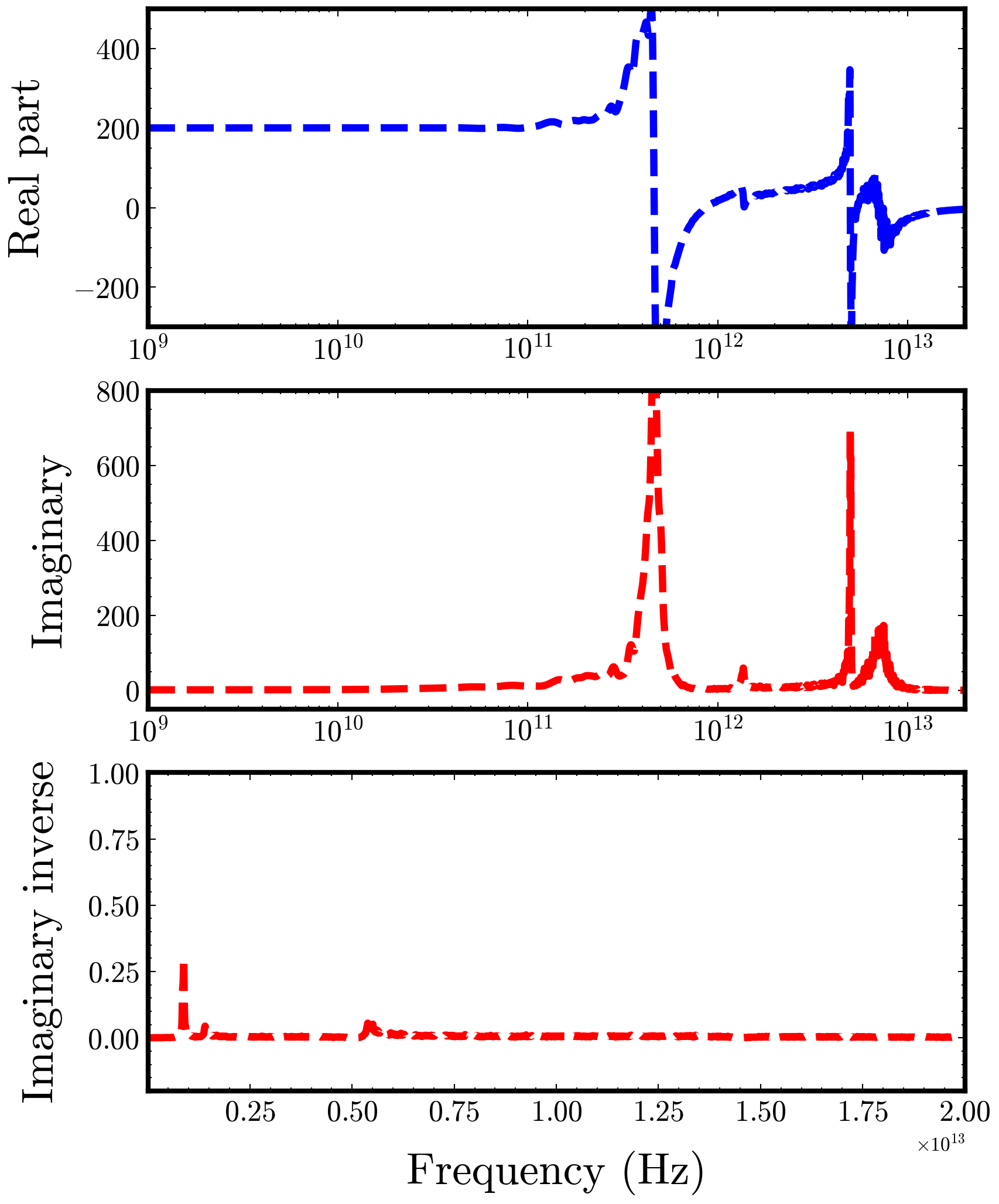
dielectric spectra results (eps2.dat && eps2.png)：

Note: Please double-check the paths and parameters in both the input files and the scripts before running. ****