Phonon spectrum calculations and QHA approximate calculation of the thermodynamic properties of materials
©️ Copyright 2025 @ Liu Theory Lab
Author:
樊迪 (Di Fan) 📨
Date:2025-8-4
Lisence:This document is licensed under Attribution-NonCommercial-ShareAlike 4.0 International (CC BY-NC-SA 4.0) license.
1 Introduction
Phonon spectrum describes the spectral distribution of lattice vibration modes (phonons) in a crystal, reflecting the vibration frequencies corresponding to different wave vectors (q). Phonons are the quantized manifestation of lattice vibrations, and their energy and momentum relationships are intuitively presented through phonon spectra. They are closely related to the thermodynamic properties (such as heat capacity and thermal conductivity) and dynamic behavior (such as phase transitions and stability) of materials. Phonopy is currently the mainstream tool for calculating phonon spectra, which calculates force constants through supercell finite displacement method or density functional perturbation theory (DFPT). It supports moving multiple atomic directions at once, significantly reducing computational complexity, and seamlessly integrates with first principles software such as VASP and QuantumESPRESSO. It can directly read output files (such as vasprun. xml) to generate force constants. The following are detailed operation steps.
2 Density Functional Perturbation Theory/Linear Response Method (DFPT)
Software that needs to be prepared: vasp+phonopy
Necessary input files:
* INCAR
* KPOINTS
* POTCAR
* band.conf
* POSCAR-unitcell(Optimized initial unit cell)
Step 1. Expand the cell to obtain the POSCAR required for computation:
Running commands directly on Linux terminals
Step 2. Submit VASP calculation:
INCAR settings are as follows:
ISMEAR =  0            (Gaussian smearing)
SIGMA  =  0.05         (Smearing value in eV)
IBRION =  8            (determines the Hessian matrix using DFPT)
EDIFF  =  1E-08        (SCF energy convergence; in eV)
PREC   =  Accurate     (Precision level)
ENCUT  =  500          (Cut-off energy for plane wave basis set, in eV)
LREAL  = .FALSE.       (Projection operators: false)
LWAVE  = .FLASE.       (Write WAVECAR or not)
LCHARG = .FLASE.       (Write CHGCAR or not)
ADDGRID= .TRUE.        (Increase grid; helps GGA convergence)
NSW    = 1
NELM   = 100
The KPOINTS file can be set as follows:
Automatic mesh
0
Gamma
2 2 2 #Here, it is generally necessary to conduct a convergence test for point K. If resources permit, point K can be set to 3 3 1, 4 4 1, etc., and the phonon spectrum can be calculated again
0 0 0
Submit VASP calculation
Step 3. Calculate phonon spectrum:
Prepare the band.conf file as follows: (See Phonopy official website for parameter meanings)
ATOM_NAME =Si #Corresponding to the element names in POSCAR.
DIM = 2 2 2 #DIM is a multiple of the cell expansion just now
BAND =0.0 0.0 0.0  0.5 0.0 0.5  0.625  0.25  0.625, 0.375 0.375 0.75  00 0.0 0.0  0.5 0.5 0.5 #It is the coordinate of a highly symmetrical point, with three coordinates in a group representing the XYZ direction. Each coordinate within a group is separated by a space, while adjacent sets of coordinates (two highly symmetrical point coordinates) are separated by two spaces.
BAND_LABELS = G K M G    #BAND_LABELS are the names of these high symmetry points.
BAND_POINTS = 101
FORCE_CONSTANTS= READ
EIGENVECTORS = .TRUE .(If you want to view the eigenvalues of the phonon spectrum, enable this option)
Step 4. Post processing steps for obtaining phonon spectra:
Run directly on the terminal ```
1. Extract the force constant and obtain the FORCEVNet file.
phonopy –fc vasprun.xml
2. Calculate the phonon spectrum and save it in PDF format
phonopy -c POSCAR-unitcell band.conf -p -s
3. Further output the phonon spectrum as a data file for drawing in other software.
Old version of phonopy
bandplot –gnuplot> phonon.txt
New version of phonopy
phonopy-bandplot –gnuplot > phonon.txt
The first line in the phonon.out file is the coordinates of the high symmetry point on the x-axis
```
3 Finite displacement method
Software that needs to be prepared: vasp+phonopy
Necessary input files:
* INCAR
* KPOINTS
* POTCAR
* band.conf
* POSCAR-unitcell(Optimized initial unit cell)
Step 1. Expand the cell to obtain the POSCAR required for computation:
Running commands directly on Linux terminals
```
1. Generate supercells
Phonopy - d - dim="2 2 2" - c POSCAR unit cell # - dim="2 2 2" represents the size of the 'x y z' expansion cell, resulting in a series of POSSCAR-001, POSSCAR-002,... numbers determined by symmetry
2. Establish a disp-* folder, with the specific quantity determined by the number of POSCAR - * generated. Put POSCAR-POTCAR, INCAR, KPOINTS into the disp - * folder
mkdir disp-001
cp POSCAR-001 ./disp-001/POSCAR
cp POTCAR ./disp-001/POTCAR
cp INCAR ./disp-001/INCAR
cp KPOINTS ./disp-001/KPOINTS
Step 2.  __Submit VASP calculation__:
INCAR settings are as follows (static calculation):
PREC = Accurate
IBRION = -1
ENCUT = 500
EDIFF = 1.0e-08
EDIFFG = -0.001
ISMEAR = 0
SIGMA = 0.05
LREAL = .FALSE.
LWAVE = .FALSE.
LCHARG = .FALSE.
KPOINTS needs to be appropriately reduced, and if possible, it is best to conduct another convergence test
Automatic mesh
0
Gamma
2 2 2 #Here, it is generally necessary to conduct a convergence test for point K. If resources permit, point K can be set to 3 3 1, 4 4 1, etc., and the phonon spectrum can be calculated again
0 0 0
```
Submit VASP calculation
Step 3. Calculate phonon spectrum:
Prepare the band.conf file as follows:
ATOM_NAME =Si
DIM = 2 2 2
BAND =0.0 0.0 0.0  0.5 0.0 0.5  0.625  0.25  0.625, 0.375 0.375 0.75  0.0 0.0 0.0  0.5 0.5 0.5
BAND_POINTS = 101
FULL_FORCE_CONSTANTS = .TRUE.
FORCE_CONSTANTS= WRITE #生成FORCE_CONSTANTS
Prepare the mesh.conf file as follows:
ATOM_NAME = Si
DIM = 2 2 2
MP = 24 24 24
Step 4. Post processing steps:
Run directly on the terminal
```
1. Extract the dynamic matrix and enter the upper level folder of disp - *
Phonopy - f./disp - */vaprun.xml # will generate FORCE SET
2. Calculate the phonon spectrum and save it in PDF format, while generating FORCEVNet
phonopy -c POSCAR-unitcell band.conf -p -s
3. Further output the phonon spectrum as a data file for drawing in other software.
Old version of phonopy
bandplot –gnuplot> phonon.txt
New version of phonopy
phonopy-bandplot –gnuplot > phonon.txt
The first line in the phonon.out file is the coordinates of the high symmetry point on the x-axis
If you have phonon spectrum data, you can also use the following Python script to draw graphs
The script is named pho. py
import numpy as np
import matplotlib as mpl
import matplotlib.pyplot as plt
plt.style.use('zty.mplstyle') #Ensure that the file path is correct
clrs = ['#6388b4', '#ef6f6a', '#55ad89', '#ffae34', '#bb7693', '#8cc2ca', '#baa094', '#c3bc3f', '#767676', '#a9b5ae']
color setting
clr1 = clrs[0]
Manually define high symmetry points and their positions
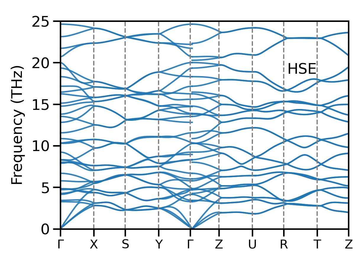
high_sym_points = ['Γ', 'X', 'S', 'Y', 'Γ', 'Z', 'U', 'R', 'T', 'Z'] high_sym_positions = np.array([0.00000000, 0.10243690, 0.19880730, 0.30124410, 0.39761450, 0.48538950, 0.58782630, 0.68419670, 0.78663360, 0.88300400])
Read phonon spectrum data from pho.dat file
with open('pho-hse.dat', 'r') as file: data = file.readlines()
Skip the first two lines (positions of high symmetry points and high symmetry points)
data = data[2:] phonon_data = [] current_data = []
for line in data: if line.strip(): points = line.split() current_data.append([float(points[0]), float(points[1])]) else: if current_data: phonon_data.append(np.array(current_data)) current_data = []
if current_data: phonon_data.append(np.array(current_data))
fig = plt.figure(figsize=(2.0, 1.48))
gs = mpl.gridspec.GridSpec(1, 1, width_ratios=[1], left=0.170, right=0.982, wspace=0,
height_ratios=[1], bottom=0.130, top=0.92, hspace=0)
ax = fig.add_subplot(gs[0])
Draw all curves
for data_set in phonon_data: wavevector = data_set[:, 0] #The first column is the wave vector frequencies = data_set[:, 1] #The second column is frequency ax.plot(wavevector, frequencies, color=clr1, alpha=0.9)
for pos in high_sym_positions: ax.axvline(x=pos, color='gray', linestyle='--', linewidth=0.5)
ax.set_xticks(high_sym_positions)
ax.set_xticklabels(high_sym_points, fontsize=7)
ax.set_ylim(0, 25)
ax.set_yticks(np.arange(0, 26, 5))
ax.set_yticklabels(np.arange(0, 26, 5), fontsize=7)
ax.set_ylabel('Frequency (THz)', fontsize=8)
ax.set_title('Phonon Dispersion', fontsize=10)
Set the x-axis display range from the first high symmetry point to the last high symmetry point
ax.set_xlim([high_sym_positions[0], high_sym_positions[-1]])
Remove gridlines
ax.grid(False)
The scale of the high symmetry point faces inward
ax.tick_params(axis='x', direction='out', length=3)
ax.tick_params(axis='y', direction='out', length=3)
Add Text
ax.text(0.89, 0.80, r'HSE', ha='right', va='top', transform=ax.transAxes, fontsize=7, color='black')
plt.subplots_adjust(left=0.17, right=0.98, bottom=0.13, top=0.98) #Fine tune the bottom and top parameters
Save Image
fig.savefig('pho-hse.jpg', dpi=600) #Save as JPG file
fig.savefig('pho-hse.pdf', dpi=600) #Save as PDF file
zty.mplstyle:storage format, change according to your own needs
1.0-column width: max 3.5 in
2.0-column width: max 7.2 in
1.5-column width: 4.72-5.36 in
figure.dpi: 600
Font
font.sans-serif: arial mathtext.fontset: custom mathtext.fallback: stixsans font.size: 6.0 # 5-7 pt
Axes
axes.facecolor: none axes.labelsize: 6.5 # 5-7 pt xtick.labelsize: 6.0 # 5-7 pt ytick.labelsize: 6.0 # 5-7 pt axes.linewidth: 0.6 # 0.25-1 pt grid.linewidth: 0.6 # 0.25-1 pt xtick.major.width: 0.6 # 0.25-1 pt ytick.major.width: 0.6 # 0.25-1 pt xtick.minor.width: 0.6 # 0.25-1 pt ytick.minor.width: 0.6 # 0.25-1 pt axes.labelpad: 2.4 # 4 * width xtick.major.size: 2.4 # 4 * width ytick.major.size: 2.4 # 4 * width xtick.minor.size: 1.8 # 3 * width ytick.minor.size: 1.8 # 3 * width xtick.major.pad: 1.2 # 2 * width ytick.major.pad: 1.2 # 2 * width
Line
lines.linewidth: 0.6 # 0.25-1 pt lines.markeredgewidth: 0.5 # 0.25-1 pt lines.markersize: 4.5
Legend
legend.facecolor: white legend.fontsize: 6.0 # 5-7 pt legend.edgecolor: C7 legend.numpoints: 2 legend.framealpha: 1.0 legend.handlelength: 1.0 legend.labelspacing: 0.3 legend.handletextpad: 0.3 legend.borderpad: 0.3 legend.borderaxespad: 0.3
```
4 QHA approximate calculation
Using phonopy to approximate the thermal properties at a certain pressure through quasi harmonic functions, including free energy, entropy, enthalpy, heat capacity, and coefficient of thermal expansion.
Step 1. Structural optimization:
Use the optimized CONTCAR as the POSCAR for the following calculation
Step 2. Establish structural files with different scaling levels:
Expand or shrink the volume of the unit cell near the equilibrium volume: increase or compress at intervals of 1%, 0.95-0.96-0.97-0.98-0.99-1.01-1.01-1.02-1.03-1.03-1.04-1.05 Create different structural files with different degrees of scaling, and place POSCAR in their respective directories one by one. You can name the folder 0.95 0.96 0.97 0.98 0.99 1.00 1.01 .....
*Note: This should be established according to your own needs (including at least 5 different degrees of scaling structures).
Step 3. Calculation of Phonon Spectrum:
Fix the volume after expansion or compression, and then perform structural optimization. Perform phonon spectrum calculations on the 11 structural files mentioned above and process them to obtain the thermalbroperence.yaml file. Here, you can refer to the calculation of phonon spectra mentioned above
Step 4. collect files:
Create mesh.conf files in each expanded or compressed folder mesh.conf: ``` ATOM_NAME = Zn 0 B DIM = 2 2 2 MP = 31 31 31 TPROP = .TRUE. TMIN = 0 TMAX = 1000 TSTEP = 10 FORCE CONSTANTS = READ
Usingphonopy - t mesh.conf ```to generate thermal_properties.yaml
Copy, paste, and collect the thermal properties. yaml files calculated and processed in each directory in the previous step into a new directory (thermal). The corresponding sequence number of the file name can be modified by yourself (for example, 1-11 can be named as thermal_properties_1.yaml, thermal_properties_2.yaml......thermal_properties_11.yaml, Corresponding to 0.95-1.05 respectively)
Step 5. Extract the volume and energy of different contraction structures to obtain the v-e.dat file:
Retrieve the volume and energy of different contraction structures (11 structures) from the directory in the third step, and collect them in the v-e.dat file. The first column is the volume, and the second column is the energy.
Step 6. Thermal properties obtained by phonopy qha treatment:
In the thermal directory, use the following command:
phonopy-qha v-e.dat thermal_properties-{1..11}.yaml
A series of. dat files can be obtained, including thermal expansion coefficient, isobaric melting, free energy, etc. These data can be imported into Origin for plotting.