The required file format is *.pbe-n-rrkjus_psl.1.0.0.UPF. The specific filename will vary.
You can download pseudopotentials from the official Quantum Espresso website (URL: http://www.quantum-espresso.org/). Navigate to PSEUDOPOTENTIALS, click on the desired element in the periodic table, find the file matching the *.pbe-n-rrkjus_psl.1.0.0.UPF format, right-click, and select "Save Link As..." to download it.
(Note: In the original document, comments were marked in blue, and parameters to be modified were in red. This has been translated into English comments.)
Important: The script may fail if it is in DOS/Windows text format, showing an error like qsub: script is written in DOS/Windows text format.
To fix this, convert the file format to Unix:
- Open the file with vi/vim: vi xxx.pbs
- In command mode, type: :set ff=unix
- Alternatively: :set fileformat=unix
- Save and quit with :wq
#!/bin/bash##PBS -q CT6#PBS -N encut # Job name#PBS -l nodes=1:ppn=36 # Modify this line and -q according to the number of cores of your machine#PBS -j oe#PBS -Vcd$PBS_O_WORKDIR# The following two lines may not be necessary for all machines# ulimit -s 40000 # ulimit -n 4096# This needs to be set to the specific installation path of the Quantum Espresso executables.# You can find this path by checking the submission scripts in a colleague's working directory.exportPW_ROOT=/home/ddf/program/espresso-5.4.0/binmkdir-p./tmp
rm-rf./tmp/*
forecin404550556065707580859095100105110115120docat>F.scf.in_$ec<< EOF&controlcalculation='scf',restart_mode='from_scratch',prefix='F' # Can be left unchanged; if modified, replace all instances of 'F' in the script.pseudo_dir = '.',outdir='./tmp'tstress=.t.,tprnfor=.t./&systemibrav = 0,celldm(1)= 1.88972688,nat= 8, # Number of atoms in the structure (count the lines under ATOMIC_POSITIONS)ntyp= 1, # Number of atomic speciesoccupations='smearing',smearing='methfessel-paxton',degauss=0.02ecutwfc=$ec,/&electronsmixing_beta = 0.7conv_thr = 1.0d-8/ATOMIC_SPECIESF 18.9984 F.pbe-n-rrkjus_psl.1.0.0.UPF # Element, Atomic Mass, Pseudopotential file# If there are other elements, add them on new lines.CELL_PARAMETERS # Structure with symmetry applied2.605373874519238 0.000000000000000 0.0000000000000000.000000000000000 2.605373874519239 0.0000000000000000.000000000000000 0.000000000000000 2.605373874519239ATOMIC_POSITIONS {crystal}F 0.0000000000000000 0.5000000000000000 0.7500000000000000F 0.0000000000000000 0.5000000000000000 -0.7500000000000000F 0.7500000000000000 0.0000000000000000 0.5000000000000001F -0.7500000000000000 0.0000000000000000 0.5000000000000000F 0.5000000000000000 0.7500000000000000 0.0000000000000000F 0.5000000000000000 -0.7500000000000001 0.0000000000000000F 0.0000000000000000 0.0000000000000000 0.0000000000000000F 0.5000000000000000 0.4999999999999999 0.5000000000000000# The above two sections are obtained from the cell file's lattice parameters.K_POINTS {automatic}12 12 12 0 0 0EOFmpirun-n36$PW_ROOT/pw.x<F.scf.in_$ec>F.scf.out_$ecdonerm-rf./tmp*
The cutoff energy can be chosen when the energy difference between consecutive steps is less than approximately 0.001 Ry. Here, we choose encut = 80 Ry.
&control
calculation='scf'
restart_mode='from_scratch',
prefix='F', # Same as before
pseudo_dir = '.',
outdir='./tmp'
/
&system
ibrav = 0,
celldm(1)=1.88972688,
nat= 8, # Same as before
ntyp= 1, # Same as before
ecutwfc=80, # Value obtained from the Encut test
ecutrho=800, # Typically 4x ecutwfc for NCPP, 10x for Ultrasoft PP
occupations='smearing',
smearing='methfessel-paxton',
degauss=0.01
la2F = .true.,
/
&electrons
conv_thr = 1.0d-8
mixing_beta = 0.7
/
ATOMIC_SPECIES
F 18.9984 F.pbe-n-rrkjus_psl.1.0.0.UPF
CELL_PARAMETERS # The structure must be symmetrized beforehand to avoid errors
2.60537300000000 0.00000000000000 0.00000000000000
0.00000000000000 2.60537300000000 0.00000000000000
0.00000000000000 0.00000000000000 2.60537300000000
ATOMIC_POSITIONS {crystal}
F 0.000000000117762 0.499999999338523 0.749986558395997
F 0.000000000339613 0.500000000256769 -0.749986558605385
F 0.749987711283413 0.000000000252767 0.499999999798142
F -0.749987712380392 0.000000000217478 0.500000000505681
F 0.500000000854287 0.749988023424662 0.000000002496860
F 0.500000000234474 -0.749988023462086 -0.000000002382903
F -0.000000000905482 -0.000000000090146 -0.000000000183659
F 0.500000000456325 0.500000000062032 0.499999999975266
K_POINTS {automatic} # A very dense mesh can be slow and hard to clean up; consider machine performance
10 10 10 0 0 0
EOF
Electron-phonon coefficients for F
&inputph
prefix='F',
fildvscf='Fdv',
amass(1)= 18.9984, # Mass of the F atom; if other atoms exist, add amass(2) = xxxx, etc.
outdir='./tmp',
fildyn='F.dyn',
electron_phonon='interpolated'
el_ph_sigma=0.005,
el_ph_nsigma=10,
trans=.true.,
ldisp=.false.
tr2_ph = 1.0d-12 /
0.000000000000000E+00 0.000000000000000E+00 0.000000000000000E+00
(3) Prepare Pseudopotential File (same as for the encut test)
# Grant permissions and submit to automatically generate a series of jobschmod+xdegauss_1.sh
./degauss_1.sh
chmod+xcpelph.sh
./cpelph.sh
chmod+xgetdate_2.sh
./getdate_2.sh
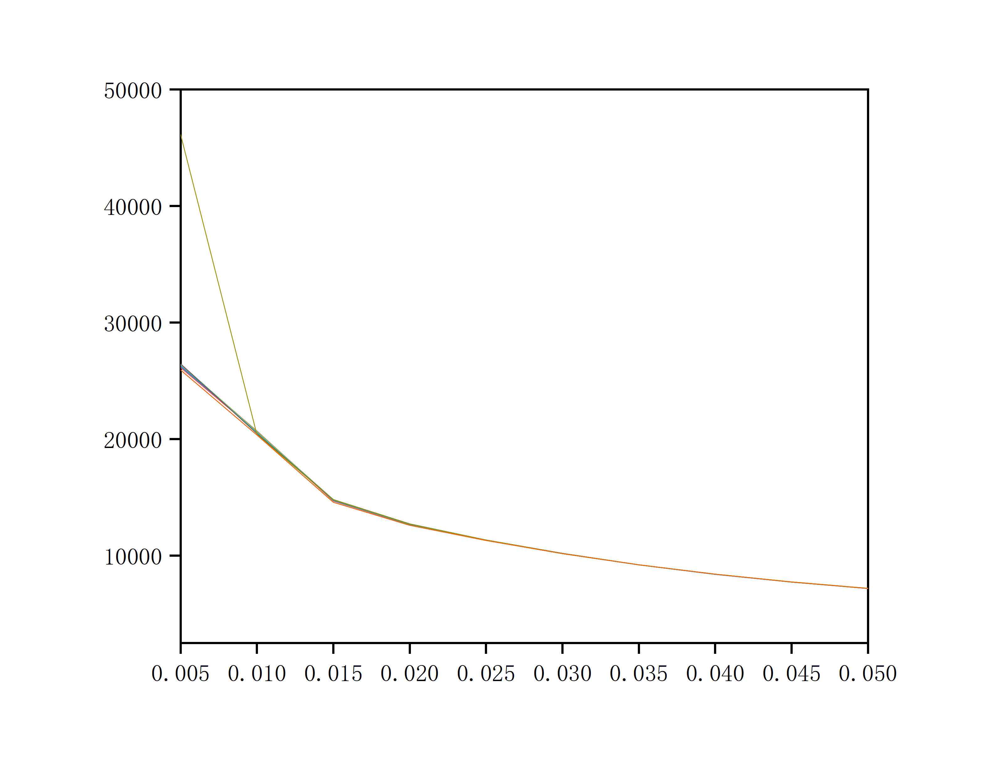
# This creates pe.txt. Import it into Origin to plot and determine the smearing width.
As shown in the figure, the smearing width is chosen as 0.03 (i.e., the position where several lines converge).
System Name
1.0
2.605373874519238 0.000000000000000 0.000000000000000
0.000000000000000 2.605373874519239 0.000000000000000
0.000000000000000 0.000000000000000 2.605373874519239
F
8
Direct
0.0000000000000000 0.5000000000000000 0.7500000000000000
...
#!/bin/bash##PBS -q CT6#PBS -N pw-opt#PBS -l nodes=1:ppn=36#PBS -j oe#PBS -Vcd$PBS_O_WORKDIRexportPW_ROOT=/share/apps/compiler/QE/espresso-5.4.0/bin/
# Add for specific servers if needed#ulimit -s 40000 #ulimit -n 4096# running programcat>F.scf.in<< EOF&controlcalculation='vc-relax',restart_mode='from_scratch',dt=30prefix='F.scf'pseudo_dir = '.',outdir='./tmp'tstress=.t.,tprnfor=.t.nstep=10000/&systemibrav = 0,celldm(1)=1.88972688nat= 8, # These four items are the same as in the smearing test scf.inntyp= 1,ecutwfc=80,ecutrho=800.occupations='smearing',smearing='mp',degauss=0.03 # Result from the smearing width testnosym = .f. # Set to .f. to apply symmetry operations/&electronsconv_thr = 1.0d-8mixing_beta = 0.7/&IONSion_dynamics = 'damp'upscale = 20/&CELLcell_dynamics = 'damp-pr'press = 30000 # Set pressure (unit: kbar, 1 kbar = 0.1 GPa)/ATOMIC_SPECIES # All below are the same as beforeF 18.9984 F.pbe-n-rrkjus_psl.1.0.0.UPFCELL_PARAMETERS2.60537300000000 0.00000000000000 0.000000000000000.00000000000000 2.60537300000000 0.000000000000000.00000000000000 0.00000000000000 2.60537300000000ATOMIC_POSITIONS {crystal}F 0.000000000117762 0.499999999338523 0.749986558395997...K_POINTS {automatic}10 10 10 0 0 0EOFmpiexec-n36$PW_ROOT/pw.x<F.scf.in>F.scf.out
The lattice parameters obtained in scf.out need to be converted back to POSCAR format. Use phonopy to apply symmetry again. (An SCF calculation might fail without applying symmetry, which can be solved by setting nosym = .f..) Then, input the final structure, in CELL format, into the subsequent SCF calculation.
The purpose of this first SCF step is threefold:
1. Determine the number of symmetry operations to verify that the symmetry is correct. Find this under the Sym. Ops. field in scf.out. (Reference for point groups vs. number of symmetry operations: http://img.chem.ucl.ac.uk/sgp/large/sgp.htm)
2. Determine the number of q-points, which corresponds to the number of .dyn files. Find this under the cart. coord. field.
3. Check the total stress to see if it corresponds to the desired pressure. Find this under the total stress field.
ii) First, import the optimized and symmetrized POSCAR into a visualization software (like VESTA or MS) to identify the high-symmetry points of the Brillouin zone.
5 # Number of high-symmetry points
20 20 20 20 # Insert 20 points in each of the 4 segments between the 5 high-symmetry points
X 0.500 0.000 0.000 # High-symmetry path
R 0.500 0.500 0.500
M 0.500 0.500 0.000
G 0.000 0.000 0.000
R 0.500 0.500 0.500
iii) Make the generator executable (chmod +x a.out) and run it (./a.out).
After execution, the specific k/q-points will be written to inp.kpt. Copy this list into the k-point section of the next scf.in file.
#!/bin/bash # Script is the same as the first SCF step#PBS -q CT1#PBS -l nodes=1:ppn=12#PBS -j oe#PBS -V#PBS -N scf-4cd$PBS_O_WORKDIRmpirun-np12/share/apps/compiler/QE/espresso-5.4.0/bin/pw.x<scf.in>scf.out
#cleanrm-rftmp
Electron-phonon coefficients for F
&inputph
prefix = 'F'
fildvscf = 'dvscf'
fildyn = 'F.dyn'
amass(1)= 18.9984,
outdir='./tmp',
electron_phonon='interpolated',
el_ph_sigma=0.05,
el_ph_nsigma=10,
alpha_mix=0.5
recover=.true.
trans=.true.,
ldisp=.true.
nq1=4, # A coarse q-point grid of 4x4x4. A value between 3-5 is common.
nq2=4, # Larger values are more accurate but slower, and can help eliminate imaginary frequencies.
nq3=4,
tr2_ph = 1.0d-12
/
Note on k-points: The list of k-points above should be taken from the output of the second SCF calculation (4-scf). Look for the section in scf.out that starts with number of k points= 81 and cart. coord. in units 2pi/alat. Be sure to use the Cartesian coordinates (cart. coord.), not the crystal coordinates. You may need to delete a column of data from what you copy.
Tip for column selection:
- Linux (vim): Press Ctrl+v (visual block mode), use arrow keys to select the column, then press d to delete.
- Windows: Paste the text into a text editor that supports block selection (like Notepad++ or VS Code) by holding Alt while selecting with the mouse.
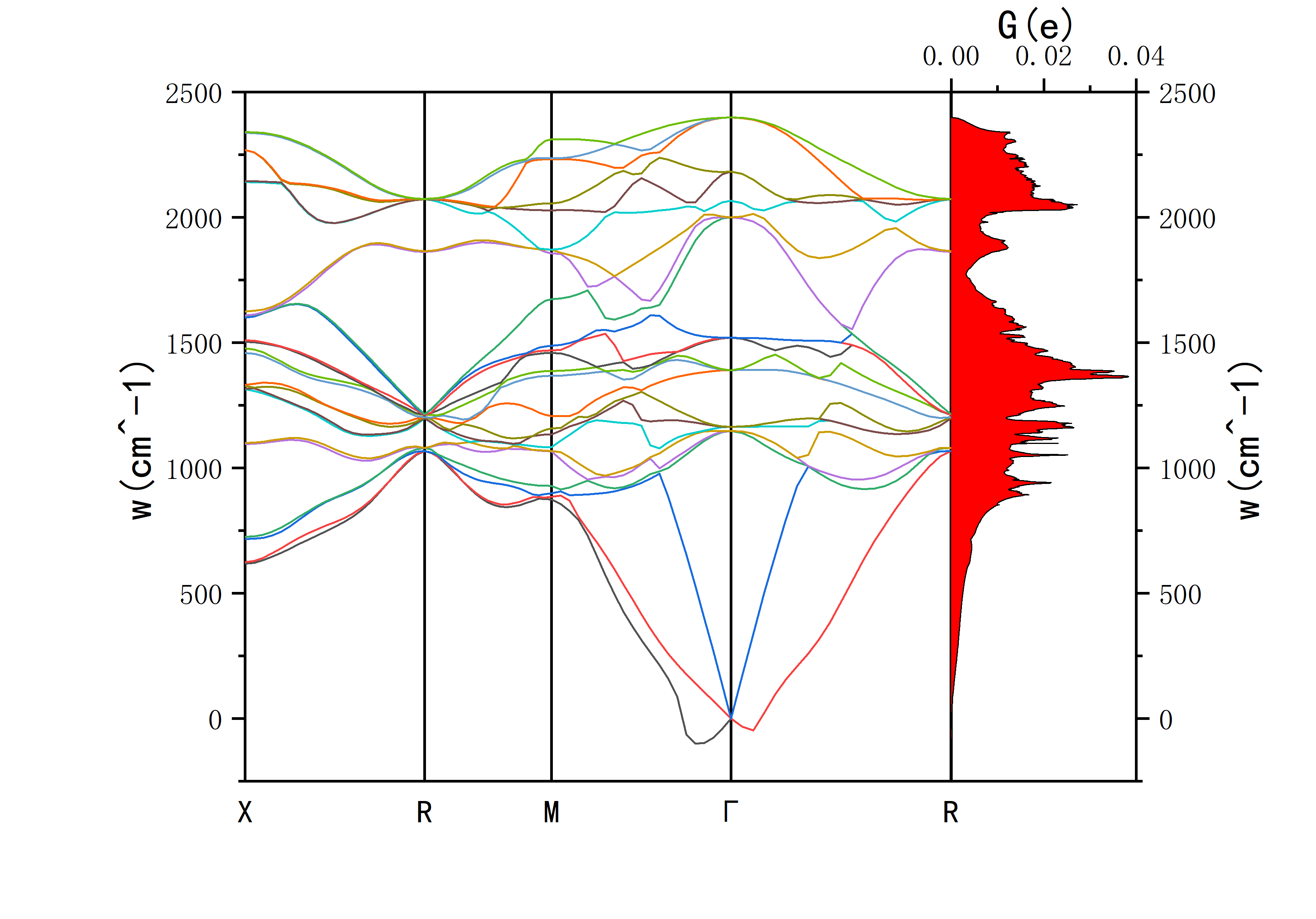
This will output the phonon spectrum and DOS data.
- F.freq.gp is used for plotting the phonon spectrum.
- phdos.dat is used for plotting the phonon density of states.
The resulting plot should look something like this:
#!/bin/shcat>lambda.in<< EOF80 0.52 1 # Line 1: [max_freq_THz] [smearing_width] [smearing_method=1]. The max frequency should be higher than the highest phonon frequency. A smearing of ~0.5 is typical.11 # Line 2: Number of k-points. Get the Cartesian k-points and weights from the first SCF step (3-scf) output file, under "cart. coord.".0.0000000 0.0000000 0.0000000 0.01600000.0000000 0.0000000 0.0766692 0.0960000...elph.inp_lambda.1elph.inp_lambda.2...elph.inp_lambda.110.13 ! mu_star, the Coulomb pseudopotential. Typically between 0.1 - 0.13.! Used in the modified Allen-Dynes formula for T_c (via omega_log)EOF/share/apps/compiler/QE/espresso-5.4.0/bin/lambda.x<lambda.in>lambda.out
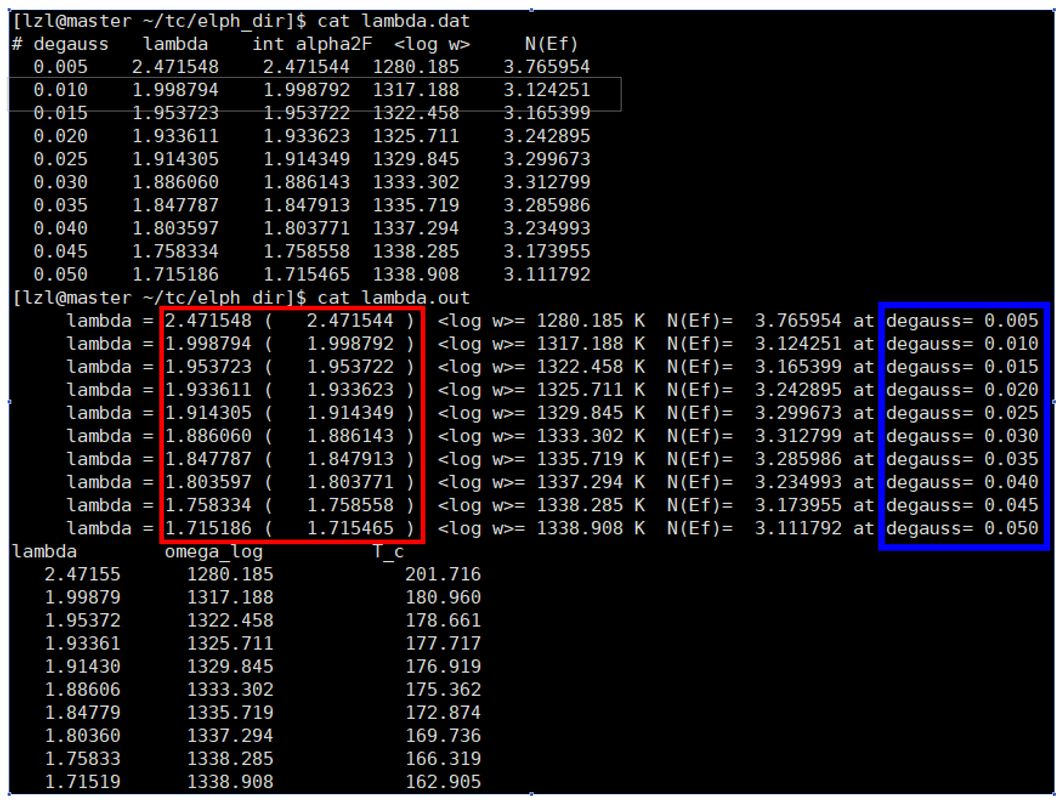
(3) Result Analysis: The calculation produces lambda.out and lambda.dat files.
In the image above, the goal is to make the values outside and inside the parentheses (in the red box) as close as possible. Ideally, they should be identical up to the last few digits. This is mainly controlled by adjusting the parameters in lambda.in. The maximum frequency value has a large impact; setting it 1-2 THz higher than the actual maximum phonon frequency is a good starting point. The smearing width also affects convergence. To determine the superconducting transition temperature (Tc), it is recommended to plot Tc versus the Gaussian broadening (blue box) in Origin to check for convergence. The converged value is the calculated Tc for the structure.