CASTEP Operation Guide
©️ Copyright 2025 @ Liu Theory Lab
Author:
Ziyue Lin 📨
Date:2025-10-20
Lisence:This document is licensed under Attribution-NonCommercial-ShareAlike 4.0 International (CC BY-NC-SA 4.0) license.
I. Basics & Bonding
(Converting cif to cell: First open .cif with MS and export .res file, then input the following command in terminal:
Simply inputting cabal will show file types that can be converted, but cannot convert directly from cif to cell.
The .cell file obtained through the above conversion is incomplete.)
The method to obtain a complete .cell file is: Open the .cif file with MS, click the three wavy lines icon - Calculation - Files - Save Files to save results to the working directory without running. The default location is: Documents - Materials Studio Projects - under a saved project. However, the .cell file is a hidden file; you need to click menu - check "Hidden items" to display it.
I. Prepare Files:
- *.usp #pseudopotential file (can be specified in .cell file in BLOCK SPECIES_POT format below)
- *.cell
- *.param
- castep.pbs.sh #declare seed_name='*' (same as *.cell filename)
1) *.cell
LATTICE_CART and POSITIONS_FRAC sections
Also need to add the following 3 items:
2) *.param
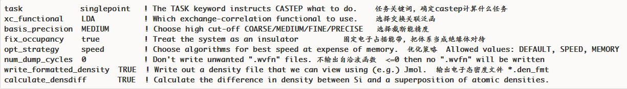
Add these two lines in *.param file to output .cell and .cif files:
Note: basis_precision cannot coexist with cut_off_energy; can only choose one, otherwise error occurs.
Also: spin_polarized - if this defaults to false, after calculation the error file .err may prompt to change to true. The reason is that spin was added to lattice parameters in .cell file. Note that only magnetic materials add spin, and initial magnetic moments may be unreasonable.
If spin is added in .cell file, write true here; if not added, write false.
II. Submit Script
Notes:
Subsequent steps (band structure, DOS, etc.) can use the following simple script:
III. Output Files: OUT.cell, OUT.castep, can be dragged into VESTA to view structure
II. Geometry Optimization (Single Pressure Point Optimization)
1. Prepare Files
1) .cell file
2) .param file
Change task name to geometry optimisation
3) castep.pbs
Can specify pressure in script or cell file
To specify optimization pressure in .cell file, format as follows:
*.param:
Notes:
Can use castep2res XXX.OUT > YYY.res command to convert results to .res file
Possible common error is:
Error check_elec_ground_state : electronic_minimisation of initial cell failed
Increase the value of MAX_SCF_CYCLES, e.g., increase to 100
III. Band Structure
(Before doing band structure, DOS, phonon spectrum with a software, need to first perform structure optimization with that software)
I. Prepare Files:
- *.cell (if in same folder, try to use different filename from previous files)
- *.param
- castep.pbs.sh
1) *.cell
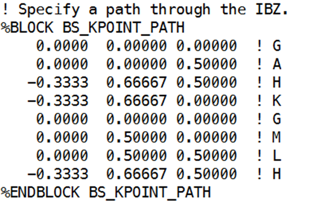
In addition to data in .cell from Basics & Bonding, also need to add Brillouin zone high-symmetry point path:
Specific operations as follows:
Export .cell file using Xftp, open with Vesta, Files – Export Data to output .cif file, then open .cif file with Material Studio, select Build – Symmetry – Find Symmetry in menu bar, click Find Symmetry button. After data appears, click Impose Symmetry in lower left to complete symmetry import.
Then select Tools – Brillouin Zone Path in menu bar, click Create to generate the path shown below:
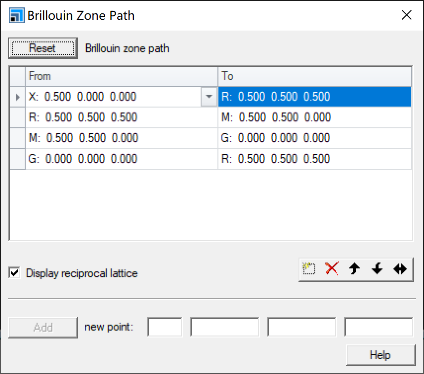
First from top to bottom, then from left to right, sequentially input in .cell file in the format shown in the image above for Brillouin Zone Path.
Note that duplicate points at corners should be omitted:
2) *.param:
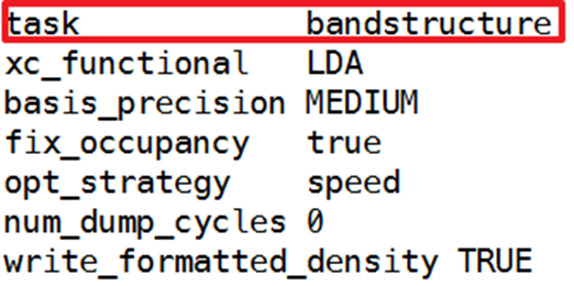
Change task name to bandstructure
xc_functional choose required pseudopotential, basis_precison same principle as before, cannot coexist with cut_off_energy
POPN_BOND_CUTOFF : 5 ang - can add this line if need to set bond length range
3) castep.pbs.sh format
II. Execute castep.pbs
Note that castep.pbs scripts obtained may contain "rm .bands" entry; adding this will automatically delete the output bands file. Remove this entry.
III. Obtain Results and Plot
Plotting Method 1:
After successful run, xxx.bands file will be output
Execute command:
After -symmetry, specify the symmetry. If no specific symmetry is given, the band structure x-axis will be numbers like -½ 0 ½ (input decimals will be converted to fractions).
How to find structure symmetry:
- Convert *.cell to .cif file using Vesta-Export Data, import .cif file to MS, Build-Symmetry-Show Symmetry (first Find Symmetry if symmetry not added) to see
Crystal System in the image above:
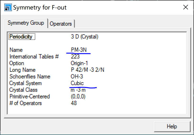
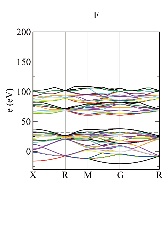
The corresponding crystal system Cubic means add -cubic after -symmetry to finally get the band structure diagram shown below:
Plotting Method 2:
Origin plotting: See details in Origin Walkthrough
IV. Density of States (DOS) Plot
I. Prepare Files
(Note that band structure results cannot be used for DOS plot; need to submit task again)
1) *.cell
Need to include
LATTICE_CART and POSITIONS_FRAC sections
But cannot add high-symmetry Brillouin zone path
2) .param same as bandstructure
II. Submit Script
dos.pl -gp *.bands uses gnuplot to plot
dos.pl -xg *.bands
Notes:
- dispersion.pl and dos.pl followed by -h can list available options
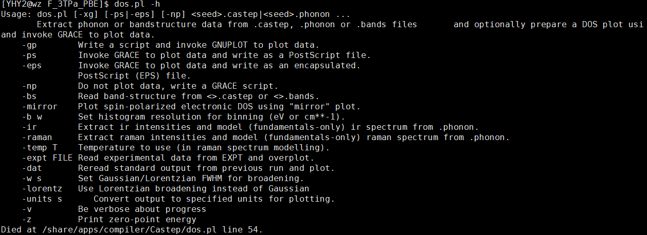
- Besides dos.pl -gp *.bands or dos.pl -xg *.bands methods to directly plot with xmanager
dos.pl directly followed by *.bands lists data needed for plotting,
dos.pl *.bands > *.txt can output as .txt file that can be plotted with Origin
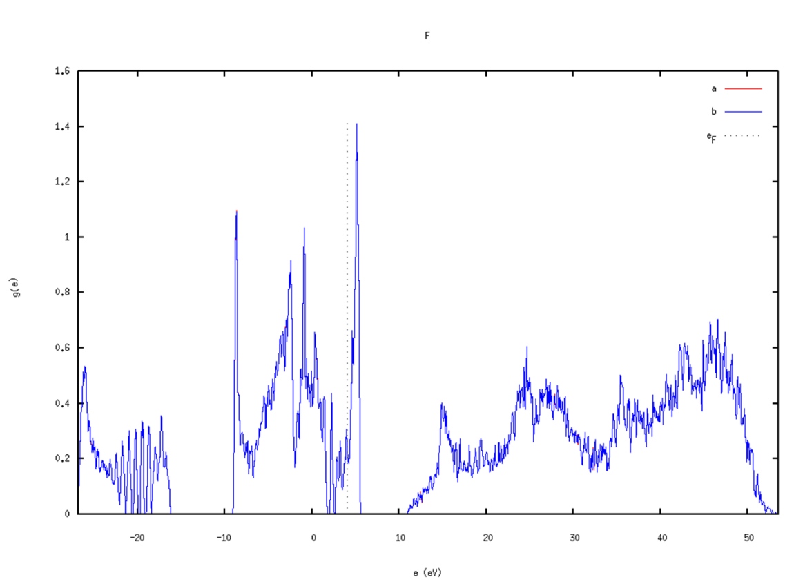
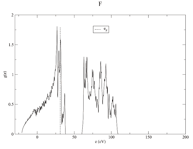
See details in Origin Walkthrough (figure integrates band structure with DOS plot)
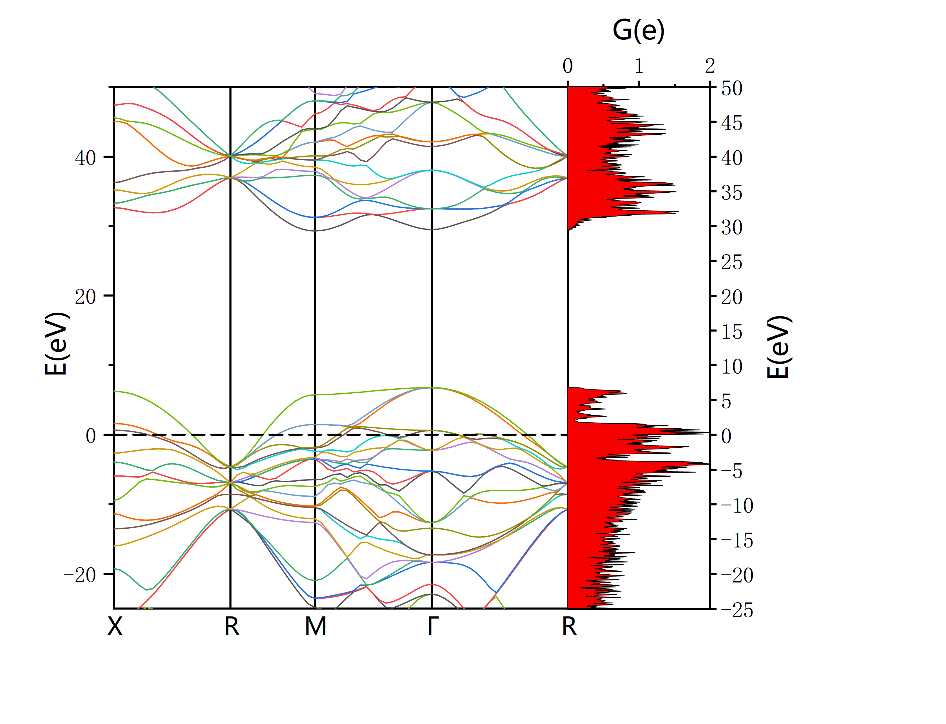
Plot by Origin
V. Phonon Spectrum Calculation
I. Prepare Files
1) *.cell
Need to include
Also need to add the following content (don't keep previous DOS and density of states parameters)
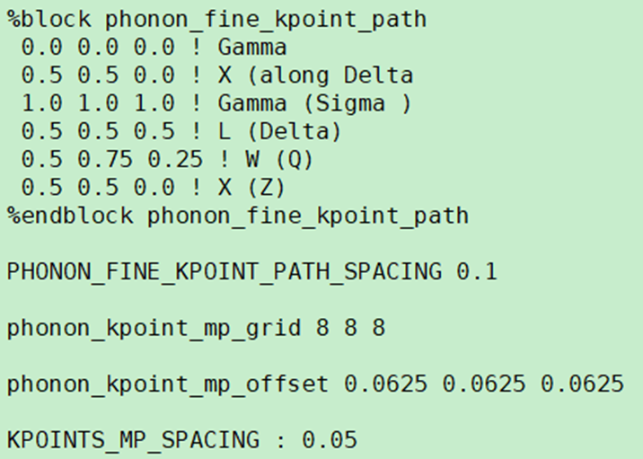
1.%block phonon_fine_kpoint_path
is the phonon q-vector path, called Dispersion path in newer MS versions
Following is the operation flow to obtain this path:
a. Import symmetry
Export optimized .cell file using Xftp, open with Vesta, Files – Export Data to output .cif file, then open .cif file with Material Studio. Select Build – Symmetry – Find Symmetry in menu bar, click Find Symmetry button. After data appears, click Impose Symmetry in lower left to complete symmetry import.
b. Obtain Brillouin zone path
i) Older Material Studio version (newer version can skip)
(See Li Mingxian CASTEP tutorial page 94, though tutorial uses MS directly for phonon spectrum)
First click three wavy lines icon-Calculation,
Select Phonon dispersion, click More… then select path
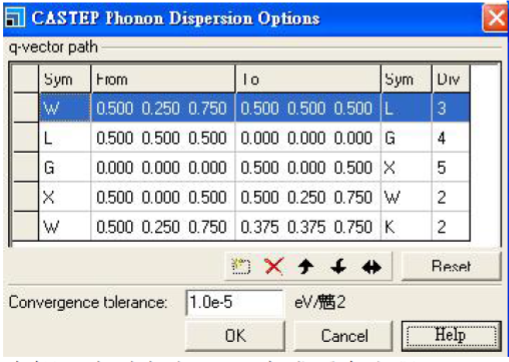
Input format see %block phonon_fine_kpoint_path section above
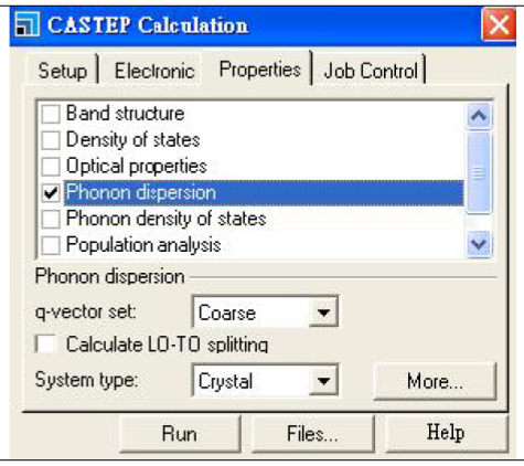
ii) Newer Material Studio version
First click three wavy lines icon-Calculation, then Properties-Phonons
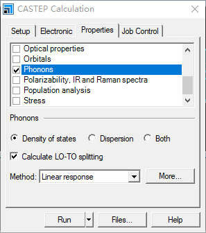
Then click More… below
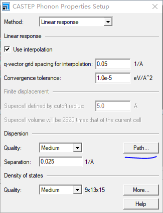
Then click Path
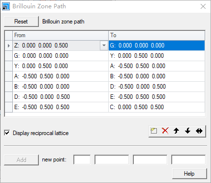
Input method same as band structure Brillouin zone path above, format see %block phonon_fine_kpoint_path section above
2. Four phonon parameters
These four phonon parameters are:
- Initial K-point spacing (can also be given as mp_grid), same as before
- High-symmetry point path grid for phonon spectrum calculation, or step size
- Phonon Brillouin zone grid, set as appropriate, use smaller values initially for calculation
- Phonon grid offset, reciprocal of twice the previous value. E.g., if Brillouin zone grid is 5, offset is 0.1
2) *.param
Change task to Phonon
Add other phonon-related items. Also remember to add MAX_SCF_CYCLES : 100, otherwise will get previous structure optimization error
3) *.pbs
Use previous simple script
F here is the filename to execute. Note that phonon spectrum input files .cell and .param need to be consistent, i.e., .OUT.cell output from previous structure optimization needs to be renamed to remove .OUT.
Then submit script.
Notes:
Common error:
Error in phonon_calculate: DFPT Linear Response not implemented for ultrasoft pseudopotentials
Ultrasoft pseudopotentials cannot directly calculate phonon spectrum.
Need to change pseudopotential or use supercell method to use ultrasoft pseudopotentials.
Specific supercell method as follows:
*.param file:
(Blue items are modifications)
Give supercell matrix in *.cell file:
Specific supercell method as follows:
After dragging .cif file into Material Studio, first import symmetry as described above.
Following is selection of unit cell or primitive cell.
In Build – Symmetry menu you can see:
Primitive Cell Conventional Cell
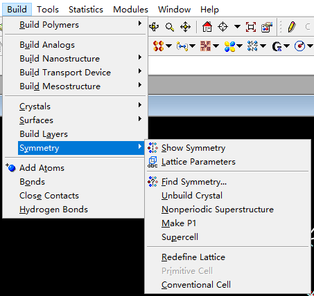
After selecting unit cell or primitive cell, Brillouin zone path and lattice parameters will differ, and supercell multiplier will also differ.
Then right-click on graphics, view Lattice Parameters (or click Lattice Parameters in image above).
Generally expand each direction to about 10 angstroms.
Plotting: dispersion.pl -xg -symmetry xxx *.phonon
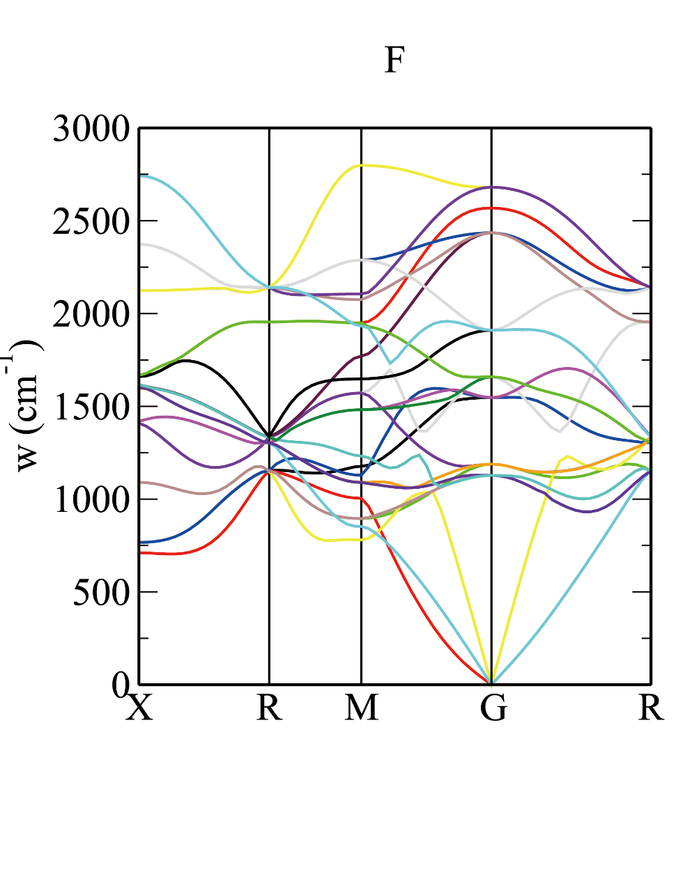
1THz=33.367cm⁻¹
VI. Projected Density of States (PDOS)
I. Prepare Files
1) *.cell
2) *.param
3) *.odi
4) *.pbs
II. Submit Script qsub F.pbs (qsub is submit command)
III. Input Command optados F
Obtain output file F.pdos.dat
IV. Plot PDOS: Note in .dat file, first column is x-axis, second and third columns are both y-axis
Plotting method basically same as DOS plot
VII. Multi-Pressure Point Structure Optimization
1) *.cell
Same as single pressure point structure optimization, input lattice parameters (can include pseudopotentials)
2) *.param
Same as single pressure point structure optimization
3) *.pbs.sh
Parts requiring modification:
Complete script in Script folder: castep_multipress.pbs.sh
Notes: CASTEP does not output .res files. If need to perform structure optimization with CASTEP results,
Use command castep2res * > *.res
(* is filename before .castep)