Calculating the Full Piezoelectric Tensor at Finite Temperature using MD¶

Author: Denan LI

Target¶

Goal: Demonstrate how to calculate the full piezoelectric tensor of a material at a finite temperature using MD simulations. We will focus on the direct method, which relies on establishing the relationship between applied stress and the resulting polarization.
After this guide: you will be able to understand the theoretical basis and the general workflow reqiured to compute a piezoelectric coefficient.
Requirement: I assume you have a working knowledge of MD code like LAMMPS.

Background¶

Piezoelectricity?¶

Piezoelectricity is the ability of a material to generate an electric charge when a mechanical force is applied. This process converts mechanical energy into electrical energy (mechanical $\rightarrow$ electricity). This phenomenon is known as the direct piezoelectric effect.

The strength of this effect is quantified by the piezoelectric coefficient, which is expressed in units of picocoulombs per newton (pC/N). This value represents the amount of charge generated per newton of applied force.

The full piezoelectric tensor?¶

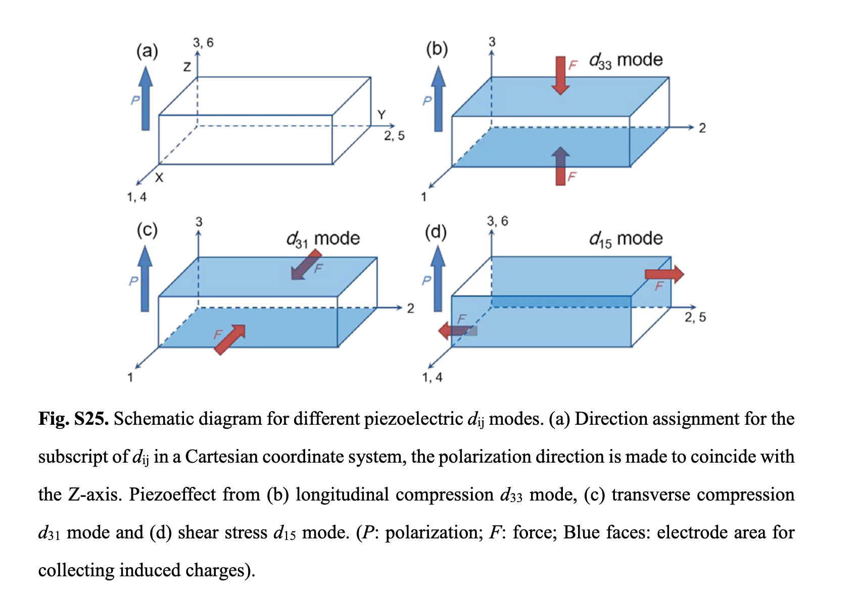
The piezoelectric coefficient is formally denoted as the tensor $d_{ij}$.

The first index, $i$ (where $i = 1, 2, 3$), indicates the direction of the resulting polarization.
The second index, $j$ (where $j = 1, 2, 3, 4, 5, 6$), specifies the direction of the applied mechanical stress using Voigt notation.

These coefficients can be represented in a matrix form:

\[d_{ij} = \begin{pmatrix} d_{11} & d_{12} & d_{13} & d_{14} & d_{15} & d_{16} \\ d_{21} & d_{22} & d_{23} & d_{24} & d_{25} & d_{26} \\ d_{31} & d_{32} & d_{33} & d_{34} & d_{35} & d_{36} \\ \end{pmatrix}\]

The figure below illustrates these different piezoelectric modes. (Source: Science 2019, 363, 1206)

alt text

How is it computed?¶

The piezoelectric coefficient can be calculated using several computational techniques.

In Density Functional Theory (DFT):
1. Density Functional Perturbation Theory (DFPT), which directly computes the response to an applied field. (e.g., J. Am. Chem. Soc. 2020, 142, 12857)
2. Finite Difference Method, which involves manually applying a series of strains/stresses and calculating the corresponding change in polarization. (e.g., J. Phys. Chem. Lett. 2016, 7, 1460)
In Molecular Dynamics (MD):
1. Inverse Effect: Applying an electric field and measuring the resulting strain to determine the piezoelectric coefficient. (e.g., Phys. Rev. Lett. 2024, 133, 046802)
2. Direct Effect: Applying a strain and measuring the change in polarization to determine the piezoelectric coefficient. (e.g., arXiv:2507.15687)

We will focus on the last method mentioned—calculating the direct piezoelectric coefficient by applying strain within an MD simulation.

MD Calculation & Results¶

Core Idea: apply the strain, measure the resulting stress and polarization change. The corresponding direct piezoelectric coefficient: $d_{ij} = \Delta P_i / \sigma_j$

Step 1: NPT simulation¶

First, we need to run a sufficiently long NPT simulation to fully relax the system. The restart file generated from this run will be used as the starting point for all subsequent calculations.

I've attached the input files used for the example system, TMCM-CdCl$_3$. Although this is a standard NPT simulation, a few key settings require attention:

# 1. Ensure all components of the pressure tensor are recorded.
thermo_style custom step temp pe ke etotal press vol lx ly lz cellalpha cellbeta cellgamma pxx pyy pzz pxy pxz pyz

# 2. Use an anisotropic barostat (`tri`) to allow all degrees of freedom of the simulation box to relax independently.
fix 2 all npt temp ${TEMP} ${TEMP} ${TAU_T} tri ${PRES} ${PRES} ${TAU_P}

Comment on simulation time: The necessary simulation time varies by material. Soft materials, like the organic-inorganic perovskite in this example, may need several nanoseconds (e.g., 5 ns) to equilibrate. In contrast, stiffer, purely inorganic systems might relax more rapidly.

It's crucial to monitor the convergence of system properties like lattice parameters and volume to determine when the system has reached a stable equilibrium.

Step 2: Apply strain¶

In LAMMPS, the simulation box is defined by six independent components: xx, yy, zz, xy, xz, and yz. The first three correspond to the box vector lengths, while the last three are the tilt factors that define the cell's shear. (For more details, see the LAMMPS documentation on triclinic boxes).

This section demonstrates how to calculate the $d_{15}$ coefficient. This corresponds to the polarization change in the x-direction ($P_1$) when a shear strain is applied in the 5-direction ($\beta$ angle of the simulation box), according to Voigt notation.

The original input file is available here. The core of the method is a standard NPT simulation embedded within a loop that incrementally applies the desired strain. The snippet below highlights the key commands:

# --- Workflow Control ---
variable i     index 1 2 3 4 5 6 7 8 9 10 
variable VALUE index -2.4 -2.1 -1.8 -1.5 -1.2 -0.9 -0.6 -0.3 -0.1 0.00
label    loop_label
# ------------------------

# --- Initialization ---
# Load the restart file from the previous step or the initial structure
variable prev equal ${i}-1
if "${i} > 1" then "read_restart restart.${prev}" &
elif "${i} == 1" "read_restart start_point.restart"
# --------------------

# --- Production Run ---
# Apply shear strain by changing the xz tilt factor
change_box      all xz final ${VALUE} remap 
write_data      init-${i}.data

# Run NPT, keeping the xz component fixed (not coupled to the barostat)
fix             2 all npt temp ${TEMP} ${TEMP} ${TAU_T} x ${PRES} ${PRES} ${TAU_P} y ${PRES} ${PRES} ${TAU_P} z ${PRES} ${PRES} ${TAU_P} xy ${PRES} ${PRES} ${TAU_P} yz ${PRES} ${PRES} ${TAU_P}

run             ${NSTEPS}
write_data      data.${i}
write_restart   restart.${i}
# --------------------

# --- Loop Control ---
clear
next i
next VALUE
jump SELF loop_label
# ------------------

Key points:

Incremental Strain: A loop is used to apply the strain in small increments. A restart file is saved after each step and used as the starting point for the next, ensuring a gradual and stable deformation.
Applying Shear Strain: The change_box command directly modifies the xz tilt factor. In this case, applying the strain essentially changes the box's $\beta$ angle from approximately 94 to 90 degrees.
Fixing the Strained Component: The xz component is intentionally omitted from the fix npt command. This decouples it from the barostat, preventing it from relaxing and thereby maintaining the applied strain during the simulation.

Step 3: Calculating Polarization¶

The method for calculating polarization depends on the system and the potential used. In this example, we use a machine learning potential that can compute dipole moments. The total polarization ($P$) is the dipole moment ($p$) divided by the simulation box volume ($V$): $P = p / V$.

To calculate the polarization for each strained state, we use the LAMMPS rerun command to process the trajectory file generated in the previous step. The original input file is available here. The key commands for this post-processing step are shown below:

# Calculate the total dipole moment using the machine learning potential
compute         dipole all deeptensor/atom dipole-fp64.pb
compute         p all reduce sum c_dipole[1] c_dipole[2] c_dipole[3]

# Convert dipole moment to polarization in units of µC/cm^2
variable        px equal "c_p[1]/vol*1602.1766208"
variable        py equal "c_p[2]/vol*1602.1766208"
variable        pz equal "c_p[3]/vol*1602.1766208"

# Configure output to the log file
thermo_style    custom step v_px v_py v_pz
thermo          1
log             ${i}.log

# Rerun the trajectory to perform the calculation
rerun           ${i}.lammpstrj every 1 dump x y z

After the rerun command finishes, the log file (e.g., ${i}.log) will contain the polarization vector at each timestep. The output will look similar to this:

   Step          v_px           v_py           v_pz     
  26000000  -3.8996057      0.028561116    4.3060153    
  26001000  -3.8665219     -0.041819721    4.159617     
  26002000  -3.8571528      0.077330292    4.4483707    
  ...

Step 4: Analysis¶

By extracting the stress and polarization data from the log files, we can calculate the piezoelectric coefficient. The Python3 script used for this purpose is available here. The key results are plotted below.

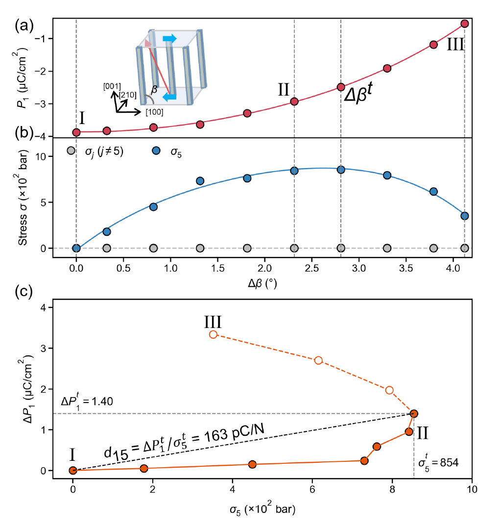
Plot of polarization and stress versus applied strain

Interpreting the Results:

Panel (a) plots the polarization ($P_1$) as a function of the applied shear strain. The trend clearly shows that as the shear strain increases ($\uparrow$), the polarization decreases ($\downarrow$).
Panel (b) shows the resulting stress as a function of strain. As expected, the dominant component is the shear stress, $\sigma_5$. The stress initially increases with strain, reaches a maximum, and then decreases. This turnover point is critical because it marks the approximate elastic limit. If strained beyond this point, the system cannot relax back to its original state even if the strain is removed.
Panel $c$ illustrates the calculation of $d_{15}$. We use the values at the critical turnover point, where the stress $\sigma_5$ reaches its maximum. This maximum stress is denoted as $\sigma_5^t$, and the corresponding change in polarization is $\Delta P_1^t$. The coefficient is then:

\[d_{15} = \frac{\Delta P_1^t}{\sigma_5^t}\]

The rationale for using this point is that experimentally measured piezoelectric coefficients describe a reproducible, elastic effect. Therefore, the calculation should be based on the maximum stress the material can withstand while still being able to return to its original state. The critical point serves as the boundary for this reversible regime.

Additional Considerations & Best Practices¶

Here are a few final points to keep in mind when performing these calculations.

1. Extracting Multiple Coefficients: While this example focused on calculating $d_{15}$, you can analyze the polarization changes in the y- and z-directions from the same simulation data to determine the $d_{25}$ and $d_{35}$ coefficients simultaneously.

2. Applying Bidirectional Strain: In practice, you should apply both positive and negative strains relative to the relaxed structure. This helps verify a linear and symmetric response in the polarization vs. stress curve, which is characteristic of the piezoelectric effect. For brevity, this guide only demonstrated applying strain in one direction.

3. Choosing an Appropriate Strain Magnitude: A key challenge is determining the right amount of strain to apply.

Too small, and the resulting changes in stress and polarization may be lost in the noise of thermal fluctuations.
Too large, and you risk pushing the material beyond its elastic limit, causing irreversible deformation.

A good approach is to test a range of strains to find a "sweet spot" that produces a measurable signal while ensuring the material's response remains elastic and reversible.

4. Calculating the Full Tensor: To compute the full piezoelectric tensor, you simply need to repeat the workflow while applying strain along the other directions (e.g., uniaxial strain for $d_{i1}$, $d_{i2}$, $d_{i3}$ or other shear strains for $d_{i4}$, $d_{i6}$). This requires modifying the change_box and fix npt commands for each case.

5. Studying Temperature Effects: Investigating how temperature impacts piezoelectricity is straightforward: just run the entire set of simulations at different target temperatures by changing the temperature variable in your LAMMPS script.

Note: Since the raw output files are large, I have not included them here. If you need them, please contact me directly (email: lidenan@westlake.edu.cn).