Oxides are typically brittle due to their strong directional ionic or covalent bonds. These bonds resist atomic glide across crystal planes, making dislocation motion more difficult and requiring significantly higher Peierls stresses than in metals. Even when atomic planes attempt to glide, the limited adaptability of the bonding network hinders rapid reconfiguration, often leading to lattice mismatch and structural failure. Consequently, oxides are prone to crack formation under mechanical stress.
Shear stress-strain curves and slip energy barriers
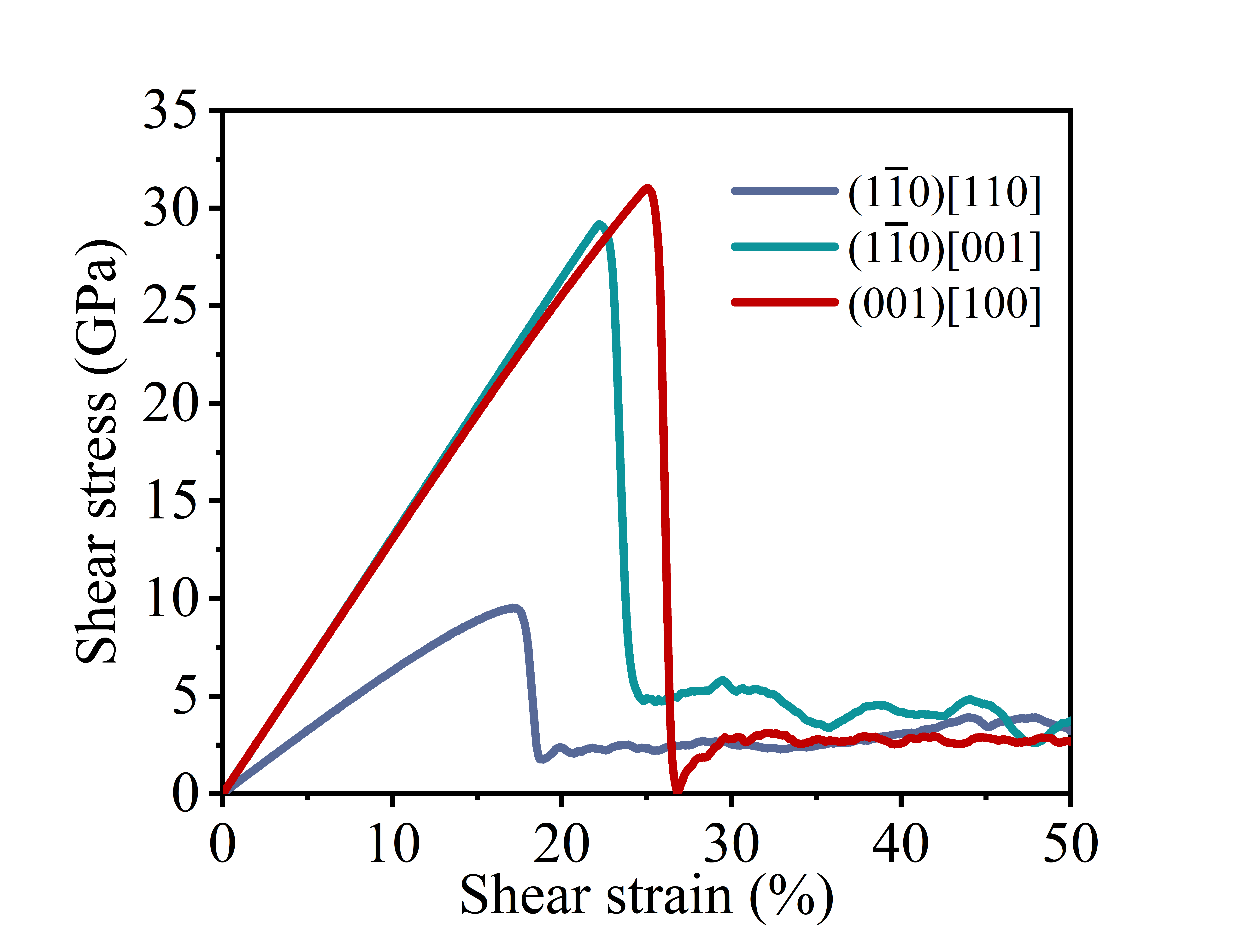
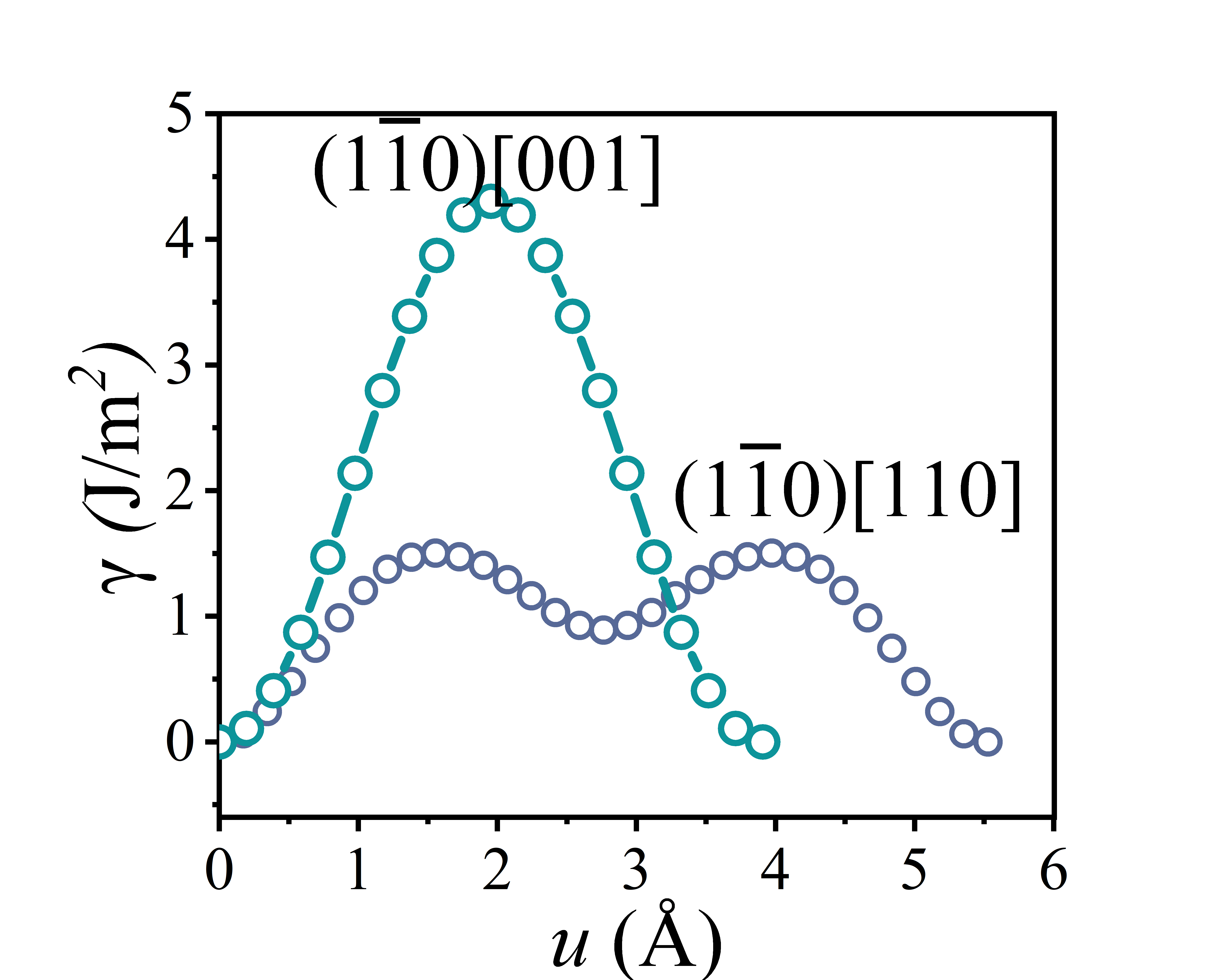
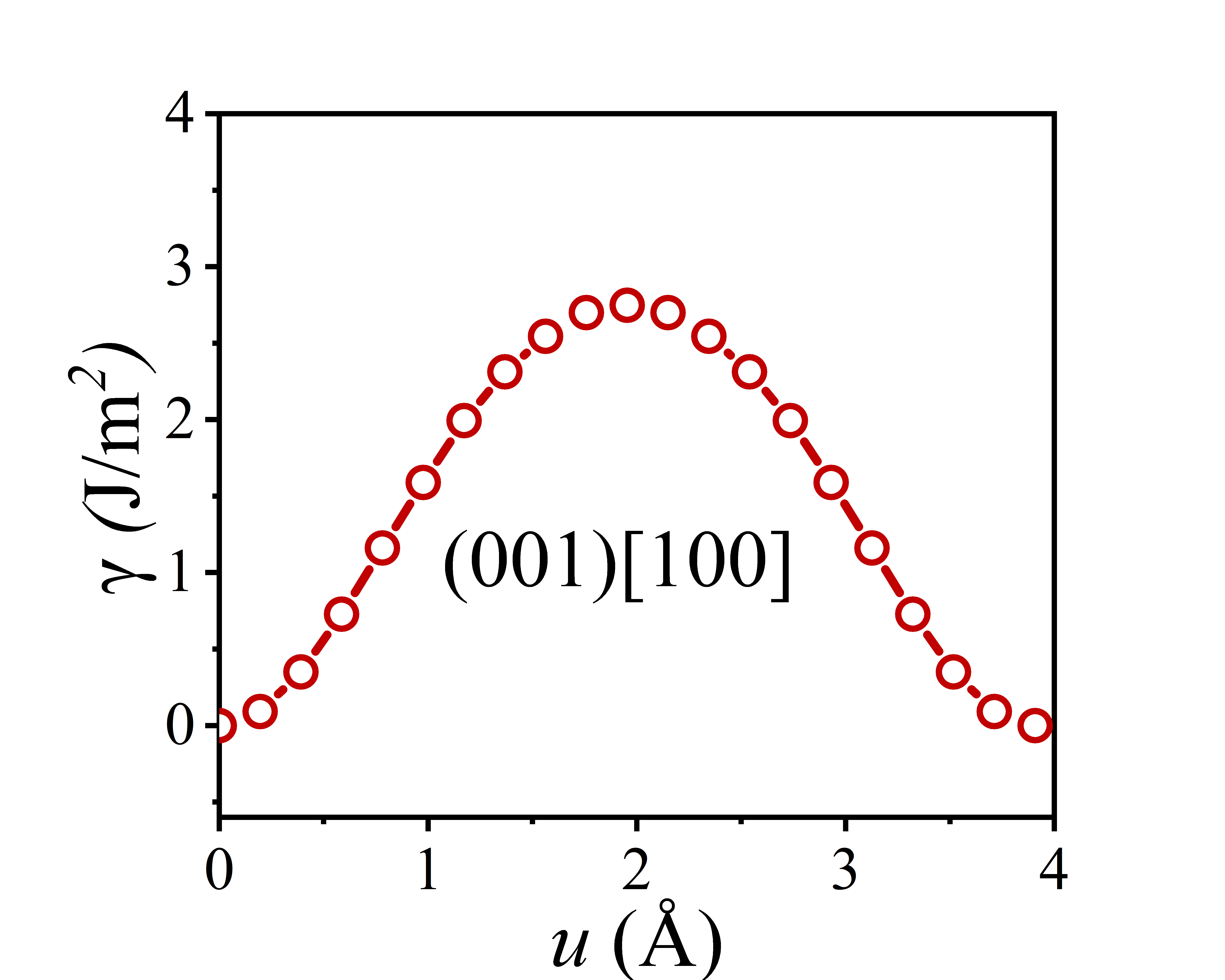
The shear stress-strain curve of a crystal provides the minimum shear stress required to activate slip systems, indicating whether dislocations can nucleate. Meanwhile, the slip energy barrier determines whether existing dislocations can glide through the crystal lattice.
Using Materials Studio, cleave and expand the MgO unit cell to create supercells along the (1-10)[110], (1-10)[001], and (001)[100] orientations. Subsequently, perform energy minimization on these three supercell structures using LAMMPS. The input file for energy minimization is shown below
#------------------------------Model settings--------------------------
clear
shell               mkdir output ./output/data

### PROGRAM PARAMETERS
units           metal

### DEFINE AND CREATE SIMULATION BOX
atom_style      atomic
##Boundary conditions (p=periodic,f=fixed)
boundary        p p p

# 输入STO-dislocation模型
read_data       conf.lmp

### ATOMS/IONS PROPERTIES
##Define atom groups
group           Mg type 1
group           O  type 2

#change_box   all triclinic
mass            1 24.305000
mass            2 15.999000

### ATOMS/IONS PROPERTIES
pair_style      deepmd MgO-compress.pb
pair_coeff      * *

#------------------------------------------- shear in xy plane -------------------------------------
variable        Temp equal 300                  # desired temperature
variable        tstp equal 0.001            # timestep
variable        tdamp equal 100*${tstp}     # damping parameters #
variable        pdamp equal 1000*${tstp}    # for NPT ensemble   #
variable        dump_every equal 100
compute         new2d all temp/partial 0 1 1
change_box      all triclinic

### PROGRAM PARAMETERS
#units           metal

### DEFINE AND CREATE SIMULATION BOX
#atom_style      charge
##Boundary conditions (p=periodic,f=fixed)
#boundary        p p p

# 输入STO-dislocation模型
#read_data           STO_relax-charge.lmp

### ATOMS/IONS PROPERTIES
##Define atom groups
### ATOMS/IONS PROPERTIES
##Define atom groups
group           Mg type 1
group           O  type 2

#change_box   all triclinic
mass            1 24.305000
mass            2 15.999000

### ATOMS/IONS PROPERTIES
pair_style      deepmd MgO-compress.pb
pair_coeff      * *


variable        tmpx equal lx
variable        tmpy equal ly
variable        tmpz equal lz
variable        L0x equal ${tmpx}
variable        L0y equal ${tmpy}
variable        L0z equal ${tmpz}

# In units metal, pressure is in [bars]; sxz is in GPa

variable        srate equal 0.01
variable        final_strain equal 1.0
variable        dyna_step equal ${final_strain}/(${srate}*${tstp})

variable        sxz equal "-pxz/10000"          # calculate shear stress
variable        strain equal ${srate}*step*${tstp}        # calculate shear strain

# deformation starts!
#fix                                1 all nve
#fix                 2 all temp/rescale 1 ${Temp} ${Temp} ${tdamp} 0.5
fix              2 all npt temp ${Temp} ${Temp} ${tdamp} iso 0.0 0.0 ${pdamp}
fix_modify       2 temp new2d

fix              3 all deform 1 xz erate ${srate} remap x
dump             1 all custom ${dump_every} STO-shear.lmp id type element x y z
dump_modify      1 sort id element Mg O
fix              def1 all print 100 "${strain} ${sxz}" file ./output/data/shear.txt screen no
thermo_style     custom step press pe pxx pyy pzz pxy pxz pyz v_strain v_sxz
run              ${dyna_step}

print "-------------------------------- All done! -----------------------------------------"
Plot the shear stress-strain curve using the shear stress-strain data obtained from the shear.txt file. The obtained shear stress-strain curve is shown in the figure below.
Visualize Slip Process in OVITO Load dump.shear.
Calculate the slip energy barrier using LAMMPS through the following procedure (SrTiO3 Example):
Construct supercell configurations with varying slip displacements.
Compute the energy of these supercells while fixing all directions except the normal to the slip plane.
The LAMMPS code for calculating the slip energy barrier is provided below:
#!/bin/bash
set -e
#source /public1/soft/modules/module.sh
#module load mpi/intel/17.0.5-cjj gcc/9.3.0-new
#export PATH=/public1/home/sch3084/test/lammps/lammps-23Jun2022/src:$PATH
#srun lmp_mpi -in sto.lin

# Check for additional files in current directory and for executables
#if [ ! -e "sto.lin" ]; then
#  printf "X!X ERROR: LAMMPS script 'sto.lin' is missing.\n"
#  exit
#fi
#if [ "$(which atomsk)" = "/public1/home/sch3084/cxk/atomsk/atomsk_b0.11.2_Linux-amd64" ]; then
#  printf "X!X ERROR: atomsk executable not found or undefined.\n"
#  exit
#fi

#if [ "$(which lmp_atom2charge.sh)" = "/public1/home/sch3084/cxk/atomsk/atomsk_b0.11.2_Linux-amd64/examples/SrTiO3_gamma_surface1" ]; then
#  printf "X!X ERROR: script lmp_atom2charge.sh not found or undefined.\n"
#  exit
#fi

#if [ "$(which charges.txt)" = "/public1/home/sch3084/ljy/atomsk/atomsk_b0.11.2_Linux-amd64/examples/SrTiO3_gamma_surface1" ]; then
#  printf "X!X ERROR: script lmp_atom2charge.sh not found or undefined.\n"
#  exit
#fi

#if [ ! -e $(which gnuplot) ]; then
#  printf "/!\ WARNING: gnuplot executable not found, no graph will be produced.\n"
#fi

# Output files
#Gamma_tau="Gamma_tau.dat"    #Whole (1-10) gamma-surface
#Gamma_100="Gamma_100.dat"    #gamma profile along [100]
#Gamma_010="Gamma_010.dat"    #gamma profile along [010]

#rm -f STO_*.lm* STO_*.out log.lammps $Gamma_tau $Gamma_100 $Gamma_010

#printf "#tauX \t tauY \t Etot_NoRelax(J/m²) \t Etot_ionRelaxed(J/m²) \n" > $Gamma_tau
#printf "#tauX \t Etot_NoRelax(J/m²) \t Etot_ionRelaxed(J/m²) \n" > $Gamma_100
#printf "#tauY \t Etot_NoRelax(J/m²) \t Etot_ionRelaxed(J/m²) \n" > $Gamma_010
# Structural parameters
alat=3.948     #lattice constant a0 of STO (A) (Thomas potential)
#S=$(echo "2.0*10*10*$alat*$alat" | bc -l)  #surface of stacking faults
#supersize=20    #Number of times the cell is repeated along Z
# Number of steps along X=[001] and Y=[110] directions
# These numbers can be increased to improve accuracy
stepX=32
stepY=20

# Use a loop to produce the different stacking faults and compute their energy

# Loop for shift along X=[001]
for ((i=0;i<=$stepX;i++)) do

  # Loop for shift along Y=[110]
  for ((j=0;j<=0;j++)) do

    # Define current shift vector tau
    tauX=$(echo "$i*$alat*sqrt(2.0)/$stepX" | bc -l)
    tauY=$(echo "$j*$alat/$stepY" | bc -l)
   # printf ">>> tau=(%.4f,%.4f). " "$tauX" "$tauY"

    # Use atomsk to create the system with stacking fault:
    # Create unit cell oriented X=[001], Y=[110], Z=[1-10]
    # Duplicate it along Z to form a supercell
    # Use the option '-shift' to build the stacking faults
    # Also use the option '-wrap' to ensure all atoms are in the box
    # Output each structure in LAMMPS data format (*.lmp)
    # Run in silent mode (-v 0)
    #printf "Building system... "
    #atomsk orient 1.lmp [100] [010] [001] -dup 10 10 $supersize lmp  >/dev/null 2>&1
    atomsk 1.lmp -shift above 0.501*BOX z $tauX $tauY 0.0 -wrap STO.lmp  >/dev/null 2>&1
    #rm orient.lmp
    atomsk STO.lmp -sort species pack POSCAR  >/dev/null 2>&1
    rm STO.lmp
    python tran.py
    rm POSCAR
    cp STO.lmp STO_${i}_${j}.lmp
    rm STO.lmp

    # Convert data file for "atom_style charge"
    #lmp_atom2charge.sh STO_${i}_${j}.lmp >/dev/null 2>&1
             #-properties charges.txt STO_${i}_${j}.lmp >/dev/null 2>&1
    # Set up the LAMMPS input script
    cp sto.lin sto_curr_${i}_${j}.lin
    sed -i "/read_data / c\read_data   STO_${i}_${j}.lmp" sto_curr_${i}_${j}.lin
    sed -i "/dump / c\dump   1 all custom 100 STO_${i}_${j}.lmc id type x y z" sto_curr_${i}_${j}.lin

    # Run LAMMPS
    #printf "Running LAMMPS... "
    #source /public1/soft/modules/module.sh
    #module load mpi/intel/17.0.5-cjj gcc/9.3.0-new
    #export PATH=/public1/home/sch3084/test/lammps/lammps-23Jun2022/src:$PATH
    #srun lmp_mpi -in sto_curr.lin
    #srun lmp_mpi -in <sto_curr.lin >/dev/null 2>&1
    #$lammps  <sto_curr.lin >/dev/null 2>&1
    #lbg job submit -i job.json -p ./ >log1
    #lmp -i sto_curr.lin >log.lammps

    # Collect energies, write them to file
    #energyNR=$(grep -A 1 "Energy initial" log.lammps | tail -n 1 | awk '{print $1}')
    #energyR=$(grep -A 1 "Energy initial" log.lammps | tail -n 1 | awk '{print $3}')
    #if [[ ( "$i" == "0" && "$j" == "0" ) ]] ; then
      #This defines the zero of energy
      #refenergyNR=$(echo "$energyNR" | bc -l)
      #refenergyR=$(echo "$energyR" | bc -l)
    #fi
    # Compute SF energy density. The factor 16.022 is to convert from eV/A² to J/m²
    #ENR=$(echo "16.022*(($energyNR)-($refenergyNR))/$S" | bc -l)
    #ER=$(echo "16.022*(($energyR)-($refenergyR))/$S" | bc -l)

    # Output results
    #printf "%.4f \t %.4f \t %.4f \t %.4f \n" "$tauX" "$tauY" "$ENR" "$ER" >> $Gamma_tau
    #if [[ "$j" == "0" ]] ; then
     # printf "%.4f \t %.4f \t %.4f \n" "$tauX" "$ENR" "$ER" >> $Gamma_100
    #fi
    #if [[ "$i" == "0" ]] ; then
     # printf "%.4f \t %.4f \t %.4f \n" "$tauY" "$ENR" "$ER" >> $Gamma_010
    #fi

    #printf "Done.\n"

    # Remove temporary files
    #rm -f sto_curr.lin log.lammps
  done

  #printf "\n" >> $Gamma_tau

done

#echo ">>> Plotting graph in EPS file 'gamma.eps'..."
#gnuplot sto.gp

#echo "\o/ Finished."
Plot the slip energy barrier curve using the data obtained from the Gamma_110.dat file. The obtained slip energy barrier curve is shown in the figure below.